Géométrie de \(\mathbb{R}^p\) : produit scalaire, distance, projection

Cours 4 — Modèles en biologie

Christophe Ambroise

L3 GBI — Université d’Évry

Acquis des cours précédents

Systèmes linéaires et pivot de Gauss

Système \(\iff\) matrice augmentée \([\,A \mid \mathbf{b}\,]\).

Opérations élémentaires sur les lignes, jusqu’à une forme échelonnée.

Pivot dans la dernière colonne	Variables libres	Solutions
oui	—	aucune
non	non	une seule
non	oui	une infinité

Produit matrice par vecteur

Combinaison des colonnes de \(A\), pondérées par les coordonnées de \(\mathbf{x}\) :

\[ A\mathbf{x} = x_1\,\mathbf{a}_1 + \dots + x_p\,\mathbf{a}_p, \qquad (A\mathbf{x})_i = \sum_{j=1}^{p} a_{ij}\, x_j \]

Dimensions : \((n \times p)\) fois \(\mathbb{R}^p\), résultat dans \(\mathbb{R}^n\).

Un système linéaire : \(A\mathbf{x} = \mathbf{b}\).

Produit matriciel, transposée, identité

\(AB = (A\mathbf{b}_1 \ \cdots \ A\mathbf{b}_q)\) ; en général \(AB \neq BA\).

\((A^T)_{ij} = a_{ji}\), \(\quad (AB)^T = B^T A^T\), \(\quad I\mathbf{x} = \mathbf{x}\).

Vecteur \(\mathbf{x} \in \mathbb{R}^p\) : une colonne, matrice \(p \times 1\). \(\mathbf{x}^T\) : une ligne, matrice \(1 \times p\).

Chaîne de Markov et vecteur propre

Évolution : \(\mathbf{x}_{t+1} = P\,\mathbf{x}_t\), \(P\) matrice de transition, colonnes de somme 1.

Équilibre : \(P\pi = \pi\), soit \((P - I)\,\pi = \mathbf{0}\) avec \(\sum_i \pi_i = 1\) ; système homogène résolu par Gauss.

Vecteur propre : \(A\mathbf{v} = \lambda\,\mathbf{v}\), \(\mathbf{v} \neq \mathbf{0}\). L’équilibre \(\pi\) : vecteur propre de \(P\) pour la valeur propre 1.

Un nuage de points

Mesures d’un individu

Un individu décrit par \(p\) mesures : un point de \(\mathbb{R}^p\).

Animal	Masse (kg)	Métabolisme (kcal/jour)
Souris	0,021	3,6
Rat	0,282	28,1
Chat	3,00	152
Chien	14,1	534
Femme	57,2	1 368
Vache	600	7 877

Métabolisme de repos, à jeun. Kleiber, Physiological Reviews, 1947, tableau 2.

Nuage de points

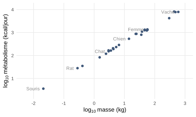
26 groupes de mammifères, de la souris à la vache. Échelle logarithmique.

Matrice des données

\(n\) individus, \(p\) variables : une matrice \(X\) de taille \(n \times p\).

\[ X = \begin{pmatrix} x_{11} & \cdots & x_{1p} \\ \vdots & & \vdots \\ x_{n1} & \cdots & x_{np} \end{pmatrix} \qquad \begin{aligned} &\text{ligne } i : \text{individu } i, \text{ un point de } \mathbb{R}^p \\ &\text{colonne } j : \text{variable } j, \text{ un vecteur de } \mathbb{R}^n \end{aligned} \]

Tableau de Kleiber : \(n = 26\), \(p = 2\).

Norme et distance

Norme en dimension 2

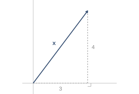
Théorème de Pythagore : \(\lVert \mathbf{x} \rVert = \sqrt{3^2 + 4^2} = 5\).

Norme dans \(\mathbb{R}^p\)

La longueur d’un vecteur : racine carrée de la somme des carrés de ses coordonnées.

\[ \lVert \mathbf{x} \rVert = \sqrt{x_1^2 + x_2^2 + \dots + x_p^2} \]

\(\lVert (1, 2, 2, 4) \rVert = \sqrt{1 + 4 + 4 + 16} = 5\).

Homogénéité : \(\lVert \alpha\,\mathbf{x} \rVert = \lvert \alpha \rvert \, \lVert \mathbf{x} \rVert\).

Distance euclidienne

La distance entre deux points : norme de leur différence.

\[ d(\mathbf{x}, \mathbf{y}) = \lVert \mathbf{x} - \mathbf{y} \rVert = \sqrt{\sum_{i=1}^{p} (x_i - y_i)^2} \]

\(\mathbf{x} = (1, 3, 2)\), \(\mathbf{y} = (4, -1, 2)\) : \(\ \mathbf{x} - \mathbf{y} = (-3, 4, 0)\), \(\ d(\mathbf{x}, \mathbf{y}) = 5\).

Vecteur unitaire

Un vecteur de norme 1.

\[ \lVert \mathbf{u} \rVert = 1, \qquad \mathbf{x} \neq \mathbf{0} \ \Rightarrow\ \frac{\mathbf{x}}{\lVert \mathbf{x} \rVert} \text{ unitaire} \]

\(\mathbf{x} = (3, 4)\) : \(\ \dfrac{\mathbf{x}}{5} = (0{,}6 ;\ 0{,}8)\).

Même direction, longueur 1.

Produit scalaire

Produit scalaire

La somme des produits des coordonnées de même rang.

\[ \mathbf{x} \cdot \mathbf{y} = \sum_{i=1}^{p} x_i\, y_i = \mathbf{x}^T \mathbf{y} \]

\(\mathbf{x}^T \mathbf{y}\) : produit d’une matrice \(1 \times p\) par une matrice \(p \times 1\).

\[ \begin{pmatrix} 1 & 2 & 3 \end{pmatrix} \begin{pmatrix} 4 \\ -5 \\ 6 \end{pmatrix} = 4 - 10 + 18 = 12 \]

Propriétés du produit scalaire

Symétrique, linéaire par rapport à chaque vecteur, et lié à la norme.

\[ \begin{aligned} &\mathbf{x} \cdot \mathbf{y} = \mathbf{y} \cdot \mathbf{x} \\ &(\mathbf{x} + \mathbf{y}) \cdot \mathbf{z} = \mathbf{x} \cdot \mathbf{z} + \mathbf{y} \cdot \mathbf{z}, \qquad (\alpha\,\mathbf{x}) \cdot \mathbf{y} = \alpha\,(\mathbf{x} \cdot \mathbf{y}) \\ &\mathbf{x} \cdot \mathbf{x} = \lVert \mathbf{x} \rVert^2 \ge 0 \end{aligned} \]

Norme d’une différence

Développement par linéarité :

\[ \begin{aligned} \lVert \mathbf{x} - \mathbf{y} \rVert^2 &= (\mathbf{x} - \mathbf{y}) \cdot (\mathbf{x} - \mathbf{y}) \\ &= \mathbf{x} \cdot \mathbf{x} - 2\,\mathbf{x} \cdot \mathbf{y} + \mathbf{y} \cdot \mathbf{y} \\ &= \lVert \mathbf{x} \rVert^2 + \lVert \mathbf{y} \rVert^2 - 2\,\mathbf{x} \cdot \mathbf{y} \end{aligned} \]

Identité algébrique, valable dans tout \(\mathbb{R}^p\).

Similarité cosinus

Le produit scalaire des deux vecteurs ramenés à la longueur 1.

\[ s(\mathbf{x}, \mathbf{y}) = \frac{\mathbf{x} \cdot \mathbf{y}}{\lVert \mathbf{x} \rVert \, \lVert \mathbf{y} \rVert} = \frac{\mathbf{x}}{\lVert \mathbf{x} \rVert} \cdot \frac{\mathbf{y}}{\lVert \mathbf{y} \rVert}, \qquad \mathbf{x} \neq \mathbf{0},\ \mathbf{y} \neq \mathbf{0} \]

Normalisation : seule compte la direction, pas la longueur.

\((1, 0)\) et \((1, 1)\) : \(\ s = \dfrac{1}{1 \times \sqrt{2}} \approx 0{,}71\).

Inégalité de Cauchy-Schwarz

Le produit scalaire de deux vecteurs est majoré, en valeur absolue, par le produit de leurs normes.

\[ \lvert \mathbf{x} \cdot \mathbf{y} \rvert \le \lVert \mathbf{x} \rVert \, \lVert \mathbf{y} \rVert \qquad \text{pour tous } \mathbf{x}, \mathbf{y} \in \mathbb{R}^p \]

Conséquence \(-1 \le s(\mathbf{x}, \mathbf{y}) \le 1\). Égalité \(s = 1\) si et seulement si \(\mathbf{y} = \lambda\,\mathbf{x}\) avec \(\lambda > 0\) ; \(s = -1\) si et seulement si \(\lambda < 0\).

Démonstration de Cauchy-Schwarz

\(\mathbf{x}\) ou \(\mathbf{y}\) nul : \(0 \le 0\). Sinon, \(\mathbf{u} = \mathbf{x} / \lVert \mathbf{x} \rVert\) et \(\mathbf{v} = \mathbf{y} / \lVert \mathbf{y} \rVert\), unitaires.

Norme d’une différence, et d’une somme :

\[ \begin{aligned} 0 \le \lVert \mathbf{u} - \mathbf{v} \rVert^2 &= 2 - 2\,\mathbf{u} \cdot \mathbf{v} \\ 0 \le \lVert \mathbf{u} + \mathbf{v} \rVert^2 &= 2 + 2\,\mathbf{u} \cdot \mathbf{v} \end{aligned} \]

D’où \(-1 \le \mathbf{u} \cdot \mathbf{v} \le 1\) ; multiplication par \(\lVert \mathbf{x} \rVert \, \lVert \mathbf{y} \rVert\) : \(\ \lvert \mathbf{x} \cdot \mathbf{y} \rvert \le \lVert \mathbf{x} \rVert \, \lVert \mathbf{y} \rVert\).

Égalité \(\mathbf{u} \cdot \mathbf{v} = 1\) : \(\lVert \mathbf{u} - \mathbf{v} \rVert = 0\), donc \(\mathbf{u} = \mathbf{v}\), même direction. \(\quad \square\)

Angle entre deux vecteurs

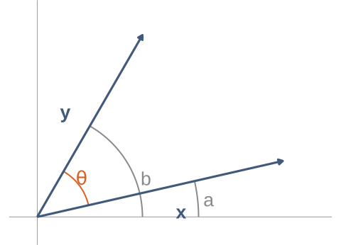
L’angle de deux vecteurs non nuls de \(\mathbb{R}^p\) : l’angle dont le cosinus est leur similarité.

\[ \theta = \arccos s(\mathbf{x}, \mathbf{y}) \in [0, \pi], \qquad \mathbf{x} \cdot \mathbf{y} = \lVert \mathbf{x} \rVert \, \lVert \mathbf{y} \rVert \cos \theta \]

Cauchy-Schwarz : \(s \in [-1, 1]\), l’arccosinus existe toujours.

\((1, 0)\) et \((1, 1)\) : \(\ \theta = \arccos \dfrac{1}{\sqrt{2}} = 45°\).

Angle dans le plan

Coordonnées polaires :

\(\mathbf{x} = \lVert \mathbf{x} \rVert (\cos a, \sin a)\)

\(\mathbf{y} = \lVert \mathbf{y} \rVert (\cos b, \sin b)\)

\[ \begin{aligned} s(\mathbf{x}, \mathbf{y}) &= \cos a \cos b + \sin a \sin b \\ &= \cos(b - a) \end{aligned} \]

\(\theta = b - a\) : l’angle usuel.

Similarité de profils

Multiplier un profil par un nombre positif ne change pas sa similarité.

\[ s(\mathbf{x}, \lambda\,\mathbf{y}) = s(\mathbf{x}, \mathbf{y}), \qquad \lambda > 0 \]

\(\mathbf{x} = (1, 2, 3)\), \(\ \mathbf{y} = (10, 20, 30) = 10\,\mathbf{x}\) : \(\ s(\mathbf{x}, \mathbf{y}) = \dfrac{140}{\sqrt{14} \times 10\sqrt{14}} = 1\), alors que \(\lVert \mathbf{y} - \mathbf{x} \rVert = 9\sqrt{14} \approx 33{,}7\).

Forme et amplitude Amplitudes très différentes, forme identique : similarité cosinus égale à 1.

Signe du produit scalaire

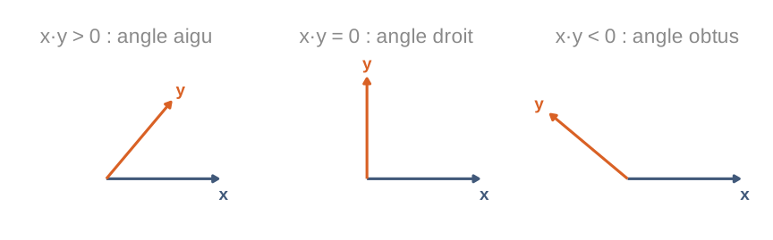
Le signe de \(\mathbf{x} \cdot \mathbf{y}\) : celui de \(s(\mathbf{x}, \mathbf{y})\), donc de \(\cos \theta\).

Orthogonalité

Vecteurs orthogonaux

Deux vecteurs dont le produit scalaire est nul.

\[ \mathbf{x} \perp \mathbf{y} \iff \mathbf{x} \cdot \mathbf{y} = 0 \]

Dans \(\mathbb{R}^4\) : \((1, 1, 0, 0) \cdot (1, -1, 2, 0) = 1 - 1 + 0 + 0 = 0\).

Un angle droit, sans dessin possible.

Théorème de Pythagore

Pour deux vecteurs orthogonaux, le carré de la norme de la somme est la somme des carrés des normes.

\[ \mathbf{x} \perp \mathbf{y} \ \Longrightarrow\ \lVert \mathbf{x} + \mathbf{y} \rVert^2 = \lVert \mathbf{x} \rVert^2 + \lVert \mathbf{y} \rVert^2 \]

Démonstration : \(\lVert \mathbf{x} + \mathbf{y} \rVert^2 = \lVert \mathbf{x} \rVert^2 + 2\,\mathbf{x} \cdot \mathbf{y} + \lVert \mathbf{y} \rVert^2\), et \(\mathbf{x} \cdot \mathbf{y} = 0\). \(\quad \square\)

Orthogonalité au vecteur \(\mathbf{1}\)

\(\mathbf{1} = (1, 1, \dots, 1) \in \mathbb{R}^n\) : \(\ \mathbf{x} \cdot \mathbf{1} = x_1 + x_2 + \dots + x_n\).

Somme nulle \(\mathbf{x} \perp \mathbf{1} \iff \displaystyle\sum_i x_i = 0 \iff \bar{x} = 0\).

Projection sur une droite

Projection d’un point sur une droite

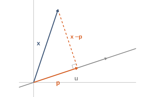
Le point de la droite le plus proche de \(\mathbf{x}\) : le pied de la perpendiculaire.

Construction de la projection

\(\mathbf{p}\) sur la droite : \(\mathbf{p} = c\,\mathbf{u}\), avec \(c\) inconnu.

Écart orthogonal à la droite :

\[ \begin{aligned} (\mathbf{x} - c\,\mathbf{u}) \cdot \mathbf{u} = 0 \ &\iff\ \mathbf{u} \cdot \mathbf{x} - c\ \mathbf{u} \cdot \mathbf{u} = 0 \\ \ &\iff\ c = \frac{\mathbf{u} \cdot \mathbf{x}}{\mathbf{u} \cdot \mathbf{u}} \end{aligned} \]

Projection orthogonale

La projection de \(\mathbf{x}\) sur la droite dirigée par \(\mathbf{u}\) : le multiple de \(\mathbf{u}\) dont l’écart à \(\mathbf{x}\) est orthogonal à \(\mathbf{u}\).

\[ \mathbf{u} \neq \mathbf{0}, \qquad \mathbf{p} = \frac{\mathbf{u}^T \mathbf{x}}{\mathbf{u}^T \mathbf{u}}\,\mathbf{u}, \qquad (\mathbf{x} - \mathbf{p}) \perp \mathbf{u} \]

\(\mathbf{u}\) unitaire : \(\ \mathbf{p} = (\mathbf{u}^T \mathbf{x})\,\mathbf{u}\).

Meilleure approximation

Aucun point de la droite n’est plus proche de \(\mathbf{x}\) que sa projection.

\[ \lVert \mathbf{x} - c\,\mathbf{u} \rVert \ \ge\ \lVert \mathbf{x} - \mathbf{p} \rVert \quad \text{pour tout } c \in \mathbb{R} \]

Démonstration : \(\mathbf{x} - c\,\mathbf{u} = (\mathbf{x} - \mathbf{p}) + (\mathbf{p} - c\,\mathbf{u})\), deux vecteurs orthogonaux. Pythagore :

\[ \lVert \mathbf{x} - c\,\mathbf{u} \rVert^2 = \lVert \mathbf{x} - \mathbf{p} \rVert^2 + \lVert \mathbf{p} - c\,\mathbf{u} \rVert^2 \ \ge\ \lVert \mathbf{x} - \mathbf{p} \rVert^2 \quad \square \]

Exemple numérique

\(\mathbf{x} = (1, 3)\), \(\ \mathbf{u} = (3, 1)\) : la figure précédente.

\[ \mathbf{u} \cdot \mathbf{x} = 3 + 3 = 6, \qquad \mathbf{u} \cdot \mathbf{u} = 10, \qquad \mathbf{p} = 0{,}6\,\mathbf{u} = (1{,}8 ;\ 0{,}6) \]

Vérification : \(\mathbf{x} - \mathbf{p} = (-0{,}8 ;\ 2{,}4)\) et \((-0{,}8) \times 3 + 2{,}4 \times 1 = 0\).

Centrage comme projection

\(\mathbf{x} = (1, 2, 3)\) projeté sur la droite dirigée par \(\mathbf{1} = (1, 1, 1)\) :

\[ \mathbf{p} = \frac{\mathbf{1} \cdot \mathbf{x}}{\mathbf{1} \cdot \mathbf{1}}\,\mathbf{1} = \frac{6}{3}\,\mathbf{1} = (2, 2, 2), \qquad \mathbf{x} - \mathbf{p} = (-1, 0, 1) \perp \mathbf{1} \]

Moyenne et centrage Projection sur \(\mathbf{1}\) : \(\ \bar{x}\,\mathbf{1}\). La moyenne est une coordonnée ; centrer, c’est retirer cette projection. \[ \mathbf{x} - \bar{x}\,\mathbf{1} \perp \mathbf{1} \]

Coordonnées d’un nuage sur un axe

Axe dirigé par \(\mathbf{u}\) unitaire : coordonnée de l’individu \(i\) \(=\) \(\mathbf{u}^T \mathbf{x}_i\). Pour tout le nuage centré : le vecteur \(X_c\mathbf{u}\).

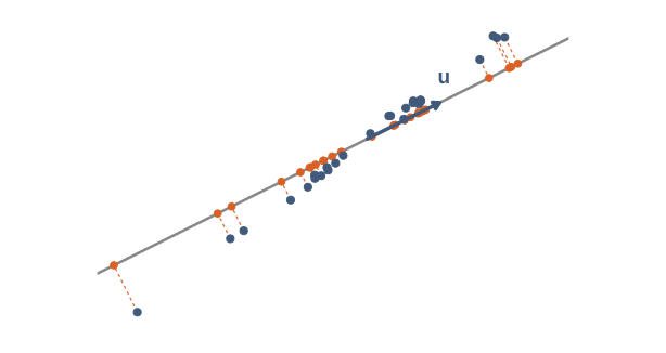
Nuage de Kleiber centré. Points bleus : individus ; points orange : leurs projections.

Droite des moindres carrés

Loi d’échelle du métabolisme

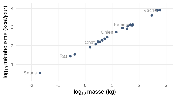
Hypothèse : \(M \approx a\,W^{b}\), soit \(\ \log M \approx \log a + b \log W\) : une droite dans le nuage.

Un système sans solution

\(x_i = \log_{10} W_i\), \(\ y_i = \log_{10} M_i\) : 26 équations, 2 inconnues.

\[ \beta_0 + \beta_1 x_i = y_i \quad (i = 1, \dots, 26) \iff X\boldsymbol\beta = \mathbf{y}, \qquad \boldsymbol\beta = \begin{pmatrix} \beta_0 \\ \beta_1 \end{pmatrix} \]

Points non alignés : système incompatible, pivot dans la dernière colonne.

Matrice \(X\) du modèle

La colonne \(\mathbf{x}\) des données, précédée d’une colonne de 1.

\[ X = \begin{pmatrix} \color{#d96125}{1} & \color{#41597a}{x_1} \\ \color{#d96125}{1} & \color{#41597a}{x_2} \\ \color{#d96125}{\vdots} & \color{#41597a}{\vdots} \\ \color{#d96125}{1} & \color{#41597a}{x_{26}} \end{pmatrix} = \bigl(\ {\color{#d96125} \mathbf{1}} \ \ {\color{#41597a} \mathbf{x}}\ \bigr), \qquad \mathbf{1}, \mathbf{x} \in \mathbb{R}^{26} \]

\[ X\boldsymbol\beta = \beta_0\,{\color{#d96125} \mathbf{1}} + \beta_1\,{\color{#41597a} \mathbf{x}} \]

Colonne \(\mathbf{1}\) : l’ordonnée à l’origine. Colonne \(\mathbf{x}\) : la pente. \(\mathbf{y}\) à part : la variable à expliquer.

Critère des moindres carrés

Chercher le \(\boldsymbol\beta\) qui rend la somme des carrés des écarts minimale.

\[ \min_{\beta_0, \beta_1}\ \sum_{i=1}^{26} (y_i - \beta_0 - \beta_1 x_i)^2 = \min_{\boldsymbol\beta}\ \lVert \mathbf{y} - X\boldsymbol\beta \rVert^2 \]

Projection orthogonale \(X\hat{\boldsymbol\beta}\) : la combinaison linéaire des colonnes de \(X\) la plus proche de \(\mathbf{y}\), c’est-à-dire la projection orthogonale de \(\mathbf{y}\) sur ces combinaisons.

Résidu orthogonal aux colonnes de \(X\)

Comme pour une droite : un résidu \(\mathbf{r} = \mathbf{y} - X\hat{\boldsymbol\beta}\) orthogonal à toutes les colonnes de \(X\).

\[ \mathbf{1}^T \mathbf{r} = 0 \ \text{ et } \ \mathbf{x}^T \mathbf{r} = 0 \iff X^T \mathbf{r} = \mathbf{0} \]

Optimalité : pour tout \(\boldsymbol\beta\), \(\ \mathbf{y} - X\boldsymbol\beta = \mathbf{r} + X(\hat{\boldsymbol\beta} - \boldsymbol\beta)\), combinaison des colonnes, donc orthogonale à \(\mathbf{r}\). Pythagore :

\[ \lVert \mathbf{y} - X\boldsymbol\beta \rVert^2 = \lVert \mathbf{r} \rVert^2 + \lVert X(\hat{\boldsymbol\beta} - \boldsymbol\beta) \rVert^2 \ \ge\ \lVert \mathbf{r} \rVert^2 \quad \square \]

Équations normales

\[ \begin{aligned} X^T \mathbf{r} = \mathbf{0} &\iff X^T (\mathbf{y} - X\hat{\boldsymbol\beta}) = \mathbf{0} \\ &\iff \boxed{X^T X\,\hat{\boldsymbol\beta} = X^T \mathbf{y}} \end{aligned} \]

Coefficients : produits scalaires entre colonnes.

\[ \begin{aligned} X^T X &= \begin{pmatrix} \mathbf{1} \cdot \mathbf{1} & \mathbf{1} \cdot \mathbf{x} \\ \mathbf{x} \cdot \mathbf{1} & \mathbf{x} \cdot \mathbf{x} \end{pmatrix} = \begin{pmatrix} 26 & 28{,}49 \\ 28{,}49 & 59{,}07 \end{pmatrix} \\[4pt] X^T \mathbf{y} &= \begin{pmatrix} \mathbf{1} \cdot \mathbf{y} \\ \mathbf{x} \cdot \mathbf{y} \end{pmatrix} = \begin{pmatrix} 69{,}03 \\ 96{,}70 \end{pmatrix} \end{aligned} \]

Résolution par le pivot de Gauss

\[ \left[\begin{array}{rr|r} 26 & 28{,}49 & 69{,}03 \\ 28{,}49 & 59{,}07 & 96{,}70 \end{array}\right] \]

\(L_2 \leftarrow L_2 - \dfrac{28{,}49}{26}\,L_1\) :

\[ \left[\begin{array}{rr|r} 26 & 28{,}49 & 69{,}03 \\ 0 & 27{,}85 & 21{,}06 \end{array}\right] \]

Remontée : \(\ \hat\beta_1 = \dfrac{21{,}06}{27{,}85} \approx 0{,}756\), \(\ \hat\beta_0 = \dfrac{69{,}03 - 28{,}49 \times 0{,}756}{26} \approx 1{,}83\).

Ajustement obtenu

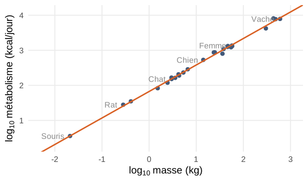
\(\log_{10} M = 1{,}83 + 0{,}756\,\log_{10} W\), la droite publiée par Kleiber.

Loi de Kleiber

\[ M \approx 67\,W^{0{,}756} \ \text{kcal/jour} \]

Exposant 3/4 Métabolisme proportionnel à la masse à la puissance \(3/4\), et non à la masse.

Par kilogramme : souris \(\approx 170\) kcal/jour, vache \(\approx 13\) kcal/jour.

M. Kleiber, Body size and metabolic rate, Physiological Reviews 27(4), 1947, p. 511–541 ; données du tableau 2, droite p. 528.