Matrices et dynamiques : chaînes de Markov

Cours 3 — Modèles en biologie

Christophe Ambroise

L3 GBI — Université d’Évry

Acquis des cours précédents

Vecteurs et combinaisons linéaires

Vecteur de \(\mathbb{R}^n\) : liste ordonnée de \(n\) nombres réels.

\[ \mathbf{x} = (x_1, \dots, x_n), \qquad \mathbf{x} + \mathbf{y}, \quad \alpha\,\mathbf{x} \ : \ \text{coordonnée par coordonnée} \]

Combinaison linéaire : \(\alpha_1 \mathbf{v}_1 + \alpha_2 \mathbf{v}_2 + \dots + \alpha_p \mathbf{v}_p\), \(\ \alpha_i \in \mathbb{R}\).

Trois lectures d’un vecteur : un profil, un état, une loi de probabilité.

Systèmes linéaires et pivot de Gauss

Système \(\iff\) matrice augmentée \([\,A \mid \mathbf{b}\,]\).

Opérations élémentaires sur les lignes, jusqu’à une forme échelonnée.

Pivot dans la dernière colonne	Variables libres	Solutions
oui	—	aucune
non	non	une seule
non	oui	une infinité

Variables libres et forme vectorielle

Variable libre : inconnue sans pivot, de valeur arbitraire.

\[ \begin{cases} x_1 = 8 + 7t \\ x_2 = 4 + 4t \\ x_3 = t \end{cases} \iff \mathbf{x} = \begin{pmatrix} 8 \\ 4 \\ 0 \end{pmatrix} + t \begin{pmatrix} 7 \\ 4 \\ 1 \end{pmatrix}, \quad t \in \mathbb{R} \]

Une infinité de solutions : un point de départ, une direction.

Un modèle à deux états

Canal ionique

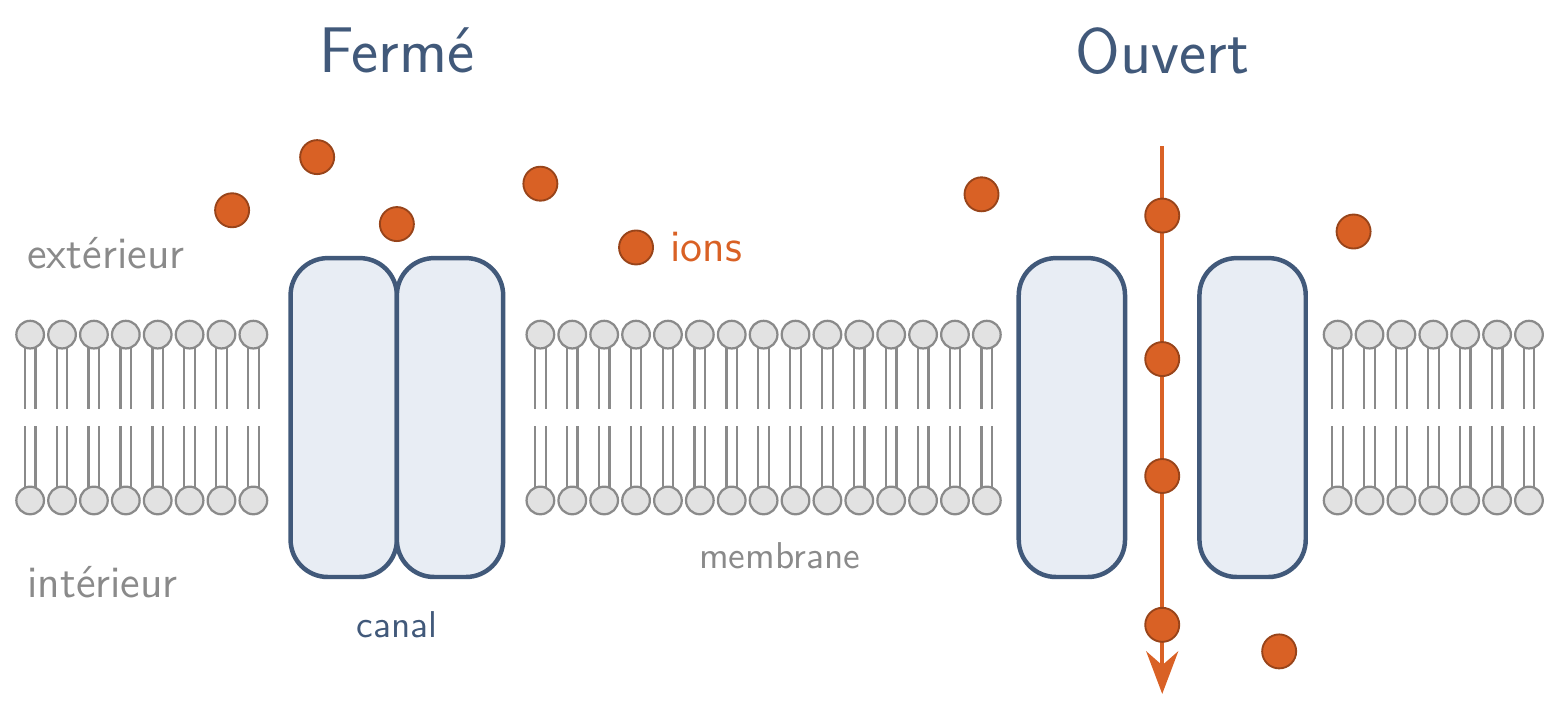
Une protéine de membrane, deux états : fermé ou ouvert.

Enregistrement d’un canal unique

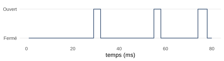
Ouvertures et fermetures au hasard, à l’échelle de la milliseconde.

Trajectoire simulée, du type de celles enregistrées en patch-clamp.

Diagramme des transitions

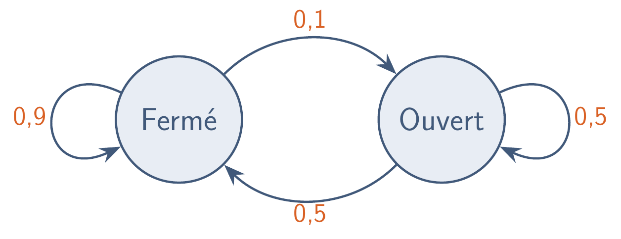
Chaque milliseconde : 1 chance sur 10 de s’ouvrir, 1 chance sur 2 de se refermer.

Propriété de Markov

L’état suivant ne dépend que de l’état présent, pas du chemin qui y a mené.

\[ \Pr(X_{t+1} = i \mid X_t = j,\ X_{t-1}, \dots, X_0) = \Pr(X_{t+1} = i \mid X_t = j) = p_{ij} \]

\(p_{ij}\) : probabilité de passer de l’état \(j\) à l’état \(i\), fixe dans le temps.

État d’un canal

Probabilités d’être fermé et d’être ouvert à l’instant \(t\) :

\[ \mathbf{x}_t = \begin{pmatrix} f_t \\ o_t \end{pmatrix}, \qquad f_t + o_t = 1 \]

Un canal : une loi de probabilité. Un million de canaux : des proportions.

Évolution en deux équations

\[ \begin{aligned} f_{t+1} &= 0{,}9\, f_t + 0{,}5\, o_t \\ o_{t+1} &= 0{,}1\, f_t + 0{,}5\, o_t \end{aligned} \]

Première ligne : loi des probabilités totales.

\[ \begin{aligned} f_{t+1} = \Pr(X_{t+1}=0) &= \Pr(X_{t+1}=0,\ X_t=0) + \Pr(X_{t+1}=0,\ X_t=1) \\ &= \Pr(X_t=0)\,\Pr(X_{t+1}=0 \mid X_t=0) \\ &\quad + \Pr(X_t=1)\,\Pr(X_{t+1}=0 \mid X_t=1) \\ &= 0{,}9\,f_t + 0{,}5\,o_t \end{aligned} \]

Fermé à \(t+1\) : resté fermé, ou refermé.

Départ fermé, \(\mathbf{x}_0 = (1 ;\ 0)\) : \(\mathbf{x}_1 = (0{,}9 ;\ 0{,}1)\).

Pas de temps et combinaison des colonnes

\[ \mathbf{x}_{t+1} = f_t \begin{pmatrix} 0{,}9 \\ 0{,}1 \end{pmatrix} + o_t \begin{pmatrix} 0{,}5 \\ 0{,}5 \end{pmatrix} \]

Premier vecteur : devenir d’un canal fermé. Second : devenir d’un canal ouvert.

Un pas de temps Une combinaison linéaire, pondérée par l’état présent.

Matrices

Matrice \(n \times p\)

Un tableau de nombres à \(n\) lignes et \(p\) colonnes.

\[ A = (a_{ij})_{\substack{1 \le i \le n \\ 1 \le j \le p}}, \qquad a_{ij} : \text{ligne } i,\ \text{colonne } j \]

\[ A = \begin{pmatrix} 2 & 0 & -1 \\ 1 & 3 & 4 \end{pmatrix} \quad : \quad 2 \times 3, \qquad a_{23} = 4 \]

Matrice carrée : \(n = p\).

Matrice de transition

Une matrice carrée à coefficients positifs, dont chaque colonne a pour somme 1.

\[ p_{ij} \ge 0 \quad \text{et} \quad \sum_{i=1}^{n} p_{ij} = 1 \quad \text{pour tout } j \]

\[ P = \begin{pmatrix} 0{,}9 & 0{,}5 \\ 0{,}1 & 0{,}5 \end{pmatrix} \]

Colonne 1 : depuis « fermé ». Colonne 2 : depuis « ouvert ».

Produit matrice par vecteur

La combinaison des colonnes de \(A\), pondérées par les coordonnées de \(\mathbf{x}\).

\[ A\mathbf{x} = x_1\,\mathbf{a}_1 + x_2\,\mathbf{a}_2 + \dots + x_p\,\mathbf{a}_p, \qquad \mathbf{a}_j = \text{colonne } j \text{ de } A \]

\(\mathbf{x}_{t+1} = f_t\,\mathbf{p}_1 + o_t\,\mathbf{p}_2\) : exactement ce produit.

Calcul ligne par ligne

Coordonnée \(i\) de \(A\mathbf{x}\) : ligne \(i\) de \(A\) et \(\mathbf{x}\), multipliées terme à terme, puis sommées.

\[ (A\mathbf{x})_i = \sum_{j=1}^{p} a_{ij}\, x_j \]

\[ \begin{pmatrix} 0{,}9 & 0{,}5 \\ 0{,}1 & 0{,}5 \end{pmatrix} \begin{pmatrix} 0{,}6 \\ 0{,}4 \end{pmatrix} = \begin{pmatrix} 0{,}9 \times 0{,}6 + 0{,}5 \times 0{,}4 \\ 0{,}1 \times 0{,}6 + 0{,}5 \times 0{,}4 \end{pmatrix} = \begin{pmatrix} 0{,}74 \\ 0{,}26 \end{pmatrix} \]

Compatibilité des dimensions

Nombre de colonnes de \(A\) \(=\) nombre de coordonnées de \(\mathbf{x}\).

\[ \underbrace{A}_{n \times p}\ \underbrace{\mathbf{x}}_{\in\, \mathbb{R}^p} \ \in\ \mathbb{R}^n \]

\(\begin{pmatrix} 2 & 0 & -1 \\ 1 & 3 & 4 \end{pmatrix} \begin{pmatrix} 1 \\ 1 \end{pmatrix}\) : non défini.

Évolution matricielle

Chaîne de Markov Un pas de temps \(=\) une multiplication par la matrice de transition. \[ \mathbf{x}_{t+1} = P\,\mathbf{x}_t \]

Écriture matricielle d’un système

Le milieu de culture du C2 :

\[ \begin{cases} 20x_1 + 10x_2 \phantom{{}+ 10x_3} = 30 \\ \phantom{2}5x_1 + 20x_2 \phantom{{}+ 10x_3} = 25 \\ \phantom{2}\;\,x_1 + \phantom{1}2x_2 + 10x_3 = 13 \end{cases} \quad \Longleftrightarrow \quad \begin{pmatrix} 20 & 10 & 0 \\ 5 & 20 & 0 \\ 1 & 2 & 10 \end{pmatrix} \begin{pmatrix} x_1 \\ x_2 \\ x_3 \end{pmatrix} = \begin{pmatrix} 30 \\ 25 \\ 13 \end{pmatrix} \]

Un système linéaire \(A\mathbf{x} = \mathbf{b}\) : quelle combinaison des colonnes de \(A\) donne \(\mathbf{b}\) ?

Plusieurs pas de temps

Deux pas enchaînés

\[ \mathbf{x}_{t+2} = P\,\mathbf{x}_{t+1} = P\,(P\,\mathbf{x}_t) \]

Une seule matrice pour deux pas : \(P\,(P\,\mathbf{x}) = (PP)\,\mathbf{x}\).

Reste à définir le produit \(PP\).

Produit de deux matrices

La matrice dont la colonne \(j\) est \(A\) multipliée par la colonne \(j\) de \(B\).

\[ AB = \bigl(A\mathbf{b}_1 \ \ A\mathbf{b}_2 \ \cdots \ A\mathbf{b}_q\bigr), \qquad (AB)_{ij} = \sum_{k=1}^{p} a_{ik}\, b_{kj} \]

Dimensions : \((n \times p)(p \times q) = n \times q\).

Calcul de \(P^2\)

\[ P^2 = \begin{pmatrix} 0{,}9 & 0{,}5 \\ 0{,}1 & 0{,}5 \end{pmatrix} \begin{pmatrix} 0{,}9 & 0{,}5 \\ 0{,}1 & 0{,}5 \end{pmatrix} = \begin{pmatrix} 0{,}86 & 0{,}70 \\ 0{,}14 & 0{,}30 \end{pmatrix} \]

\((P^2)_{21} = 0{,}1 \times 0{,}9 + 0{,}5 \times 0{,}1 = 0{,}14\)

Fermé → fermé → ouvert, ou fermé → ouvert → ouvert.

\((P^2)_{ij}\) : probabilité de passer de \(j\) à \(i\) en deux pas.

Non-commutativité

\[ \begin{aligned} \begin{pmatrix} 1 & 1 \\ 0 & 1 \end{pmatrix} \begin{pmatrix} 1 & 0 \\ 1 & 1 \end{pmatrix} &= \begin{pmatrix} 2 & 1 \\ 1 & 1 \end{pmatrix} \\[4pt] \begin{pmatrix} 1 & 0 \\ 1 & 1 \end{pmatrix} \begin{pmatrix} 1 & 1 \\ 0 & 1 \end{pmatrix} &= \begin{pmatrix} 1 & 1 \\ 1 & 2 \end{pmatrix} \end{aligned} \]

Ordre des facteurs En général, \(AB \neq BA\).

Puissances d’une matrice

\[ P^t = \underbrace{P\,P \cdots P}_{t \text{ facteurs}}, \qquad \mathbf{x}_t = P^t\,\mathbf{x}_0 \]

\((P^t)_{ij}\) : probabilité de passer de \(j\) à \(i\) en \(t\) pas.

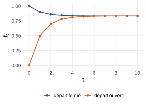
Convergence observée

\(t\)	\(f_t\), départ fermé	\(f_t\), départ ouvert
0	1	0
1	0,9	0,5
2	0,86	0,7
3	0,844	0,78
4	0,838	0,812
5	0,835	0,825

Oubli de l’état initial

Même limite Départ fermé ou départ ouvert : \(\mathbf{x}_t \to (5/6 ;\ 1/6)\).

Cette limite : comment la calculer ? Existe-t-elle pour toute chaîne ?

Distribution d’équilibre

Distribution d’équilibre

Une loi de probabilité que la chaîne laisse inchangée.

\[ P\pi = \pi, \qquad \pi_i \ge 0, \qquad \sum_{i} \pi_i = 1 \]

Matrice identité et système homogène

Matrice identité \(I\) : des 1 sur la diagonale, des 0 ailleurs. \(I\mathbf{x} = \mathbf{x}\).

\[ P\pi = \pi \iff P\pi - I\pi = \mathbf{0} \iff (P - I)\,\pi = \mathbf{0} \]

\(P - I\) : soustraction coefficient par coefficient.

Système homogène : second membre nul. Toujours la solution \(\pi = \mathbf{0}\).

Rôle de la contrainte \(\sum_i \pi_i = 1\) écarte la solution nulle.

Équilibre du canal ionique

\[ P - I = \begin{pmatrix} -0{,}1 & 0{,}5 \\ 0{,}1 & -0{,}5 \end{pmatrix} \]

Deux lignes opposées : une seule équation, \(-0{,}1\,f + 0{,}5\,o = 0\), soit \(f = 5\,o\). Variable libre : \(o\).

Avec \(f + o = 1\) : \(\pi = (5/6 ;\ 1/6)\).

Probabilité d’ouverture Canal ouvert un sixième du temps.

Succession écologique à trois états

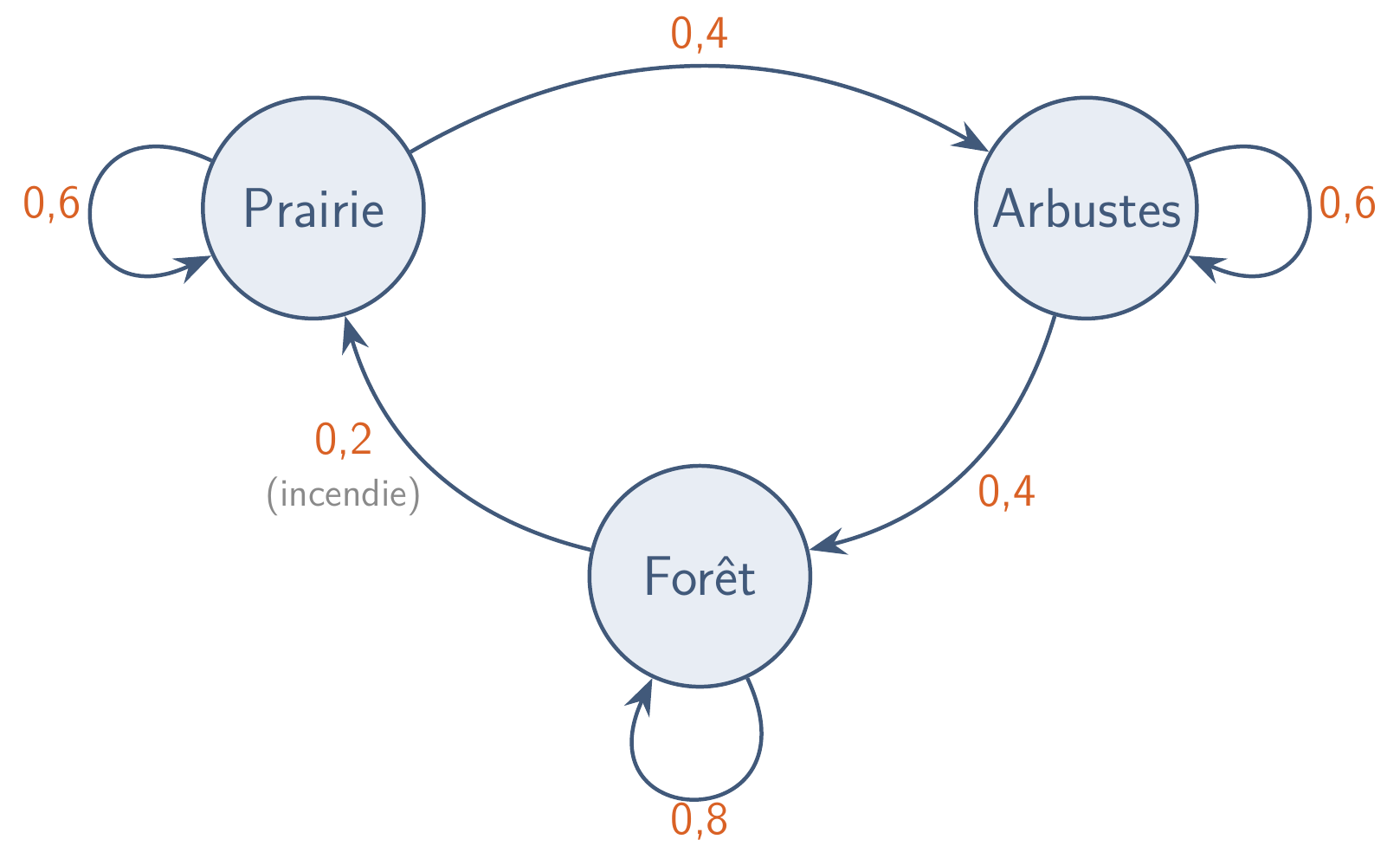
Pas de temps : une décennie. Incendie : retour de la forêt à la prairie.

Pivot de Gauss sur \(P - I\)

\[ P = \begin{pmatrix} 0{,}6 & 0 & 0{,}2 \\ 0{,}4 & 0{,}6 & 0 \\ 0 & 0{,}4 & 0{,}8 \end{pmatrix}, \qquad 5\,(P - I) = \begin{pmatrix} -2 & 0 & 1 \\ 2 & -2 & 0 \\ 0 & 2 & -1 \end{pmatrix} \]

\(L_2 \leftarrow L_2 + L_1\), puis \(L_3 \leftarrow L_3 + L_2\) :

\[ \begin{pmatrix} -2 & 0 & 1 \\ 0 & -2 & 1 \\ 0 & 0 & 0 \end{pmatrix} \]

Ligne nulle : \(\pi_3\) libre.

Équilibre du paysage

\[ \begin{aligned} -2\pi_1 + \pi_3 = 0 \quad &\Rightarrow \quad \pi_1 = \pi_3 / 2 \\ -2\pi_2 + \pi_3 = 0 \quad &\Rightarrow \quad \pi_2 = \pi_3 / 2 \end{aligned} \]

\(\pi_1 + \pi_2 + \pi_3 = 2\,\pi_3 = 1\) : \(\pi = (1/4 ;\ 1/4 ;\ 1/2)\).

À long terme Un quart de prairie, un quart d’arbustes, la moitié en forêt.

Vecteur propre

Vecteur propre, valeur propre

Un vecteur non nul que la matrice transforme en un multiple de lui-même ; le facteur est la valeur propre.

\[ A \text{ carrée}, \qquad A\mathbf{v} = \lambda\,\mathbf{v}, \qquad \mathbf{v} \neq \mathbf{0}, \quad \lambda \in \mathbb{R} \]

Un état que le modèle reproduit, à un facteur près.

L’équilibre comme vecteur propre

\[ P\pi = \pi = 1 \cdot \pi \]

Équilibre Un vecteur propre de \(P\), associé à la valeur propre 1.

Second vecteur propre du canal

\[ P \begin{pmatrix} 1 \\ -1 \end{pmatrix} = \begin{pmatrix} 0{,}9 - 0{,}5 \\ 0{,}1 - 0{,}5 \end{pmatrix} = \begin{pmatrix} 0{,}4 \\ -0{,}4 \end{pmatrix} = 0{,}4 \begin{pmatrix} 1 \\ -1 \end{pmatrix} \]

\(\mathbf{v} = (1 ;\ -1)\) : vecteur propre, valeur propre \(0{,}4\).

\[ \mathbf{v} = \begin{pmatrix}1\\0\end{pmatrix} - \begin{pmatrix}0\\1\end{pmatrix} \]

Pas une loi : l’excès de fermé sur ouvert, un déséquilibre.

Vitesse de convergence

Départ fermé : \(\mathbf{x}_0 = (1 ;\ 0) = \pi + \tfrac16\,\mathbf{v}\).

Linéarité, \(P(\mathbf{u} + c\,\mathbf{v}) = P\mathbf{u} + c\,P\mathbf{v}\) :

\[ \mathbf{x}_t = P^t\pi + \tfrac16\,P^t\mathbf{v} = \pi + \tfrac16\,(0{,}4)^t\,\mathbf{v} \]

Seconde valeur propre Écart à l’équilibre multiplié par \(0{,}4\) à chaque pas.

Seconde valeur propre et mélange

Toute loi initiale : \(\mathbf{x}_0 = \pi + c\,\mathbf{v}\) — l’équilibre plus un déséquilibre \(c\).

\(\lambda_2 = 0{,}4\) : ce déséquilibre multiplié par \(0{,}4\) à chaque pas.

\(0{,}4^5 \approx 0{,}01\) : après cinq pas, \(1\,\%\) du déséquilibre initial. Le tableau : \(f_5 = 0{,}835\), à \(0{,}002\) de l’équilibre.

Vitesse de mélange \(\lambda_2\) proche de \(1\) : oubli lent ; proche de \(0\) : oubli rapide.

Théorème de Perron-Frobenius

Théorème de Perron-Frobenius

Une chaîne à nombre fini d’états, à probabilités de transition fixes, où tout état est accessible depuis tout autre et sans cycle fixe, possède une unique distribution d’équilibre, limite de la chaîne quel que soit l’état initial.

\[ \exists!\ \pi : \ P\pi = \pi,\ \ \sum_i \pi_i = 1 \qquad \text{et} \qquad P^t\,\mathbf{x}_0 \xrightarrow[t \to \infty]{} \pi \ \text{ pour toute loi initiale } \mathbf{x}_0 \]

Chaîne irréductible et apériodique. Scott E. Page, The Model Thinker, ch. 17.

Hypothèses non satisfaites

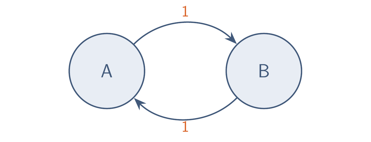
Cycle fixe — oscillation sans fin ; équilibre \((1/2 ;\ 1/2)\) jamais atteint.

\[ P = \begin{pmatrix} 0 & 1 \\ 1 & 0 \end{pmatrix} \]

États isolés — \(P = I\) : aucun passage d’un état à l’autre. \(P\pi = \pi\) pour toute loi : une infinité d’équilibres.

Équilibre et intervention

Ouvrir des canaux, un instant : retour au même équilibre.

Un médicament qui double la probabilité de s’ouvrir, de \(0{,}1\) à \(0{,}2\) :

\[ P' = \begin{pmatrix} 0{,}8 & 0{,}5 \\ 0{,}2 & 0{,}5 \end{pmatrix}, \qquad \pi' = (5/7 ;\ 2/7) \]

Équilibre Déterminé par les probabilités de transition.

Transposée

La matrice obtenue en échangeant lignes et colonnes.

\[ (A^T)_{ij} = a_{ji}, \qquad \begin{pmatrix} 2 & 0 & -1 \\ 1 & 3 & 4 \end{pmatrix}^{T} = \begin{pmatrix} 2 & 1 \\ 0 & 3 \\ -1 & 4 \end{pmatrix} \]

Transposée d’un produit : \((AB)^T = B^T A^T\).

Convention en lignes

Dans de nombreux livres et logiciels : état en ligne, lignes de somme 1.

\[ Q = P^T = \begin{pmatrix} 0{,}9 & 0{,}1 \\ 0{,}5 & 0{,}5 \end{pmatrix}, \qquad \mathbf{x}_{t+1}^T = (P\mathbf{x}_t)^T = \mathbf{x}_t^T\, Q \]

Équilibre : \(\pi^T Q = \pi^T\).

Deux écritures Même modèle. Dans ce cours : état en colonne, \(\mathbf{x}_{t+1} = P\mathbf{x}_t\).