Analyse en composantes principales

Séance 6 — Projection, reconstruction et inertie

Christophe Ambroise

UEVE, UMR CNRS 8071

19 octobre 2026

Un modèle latent

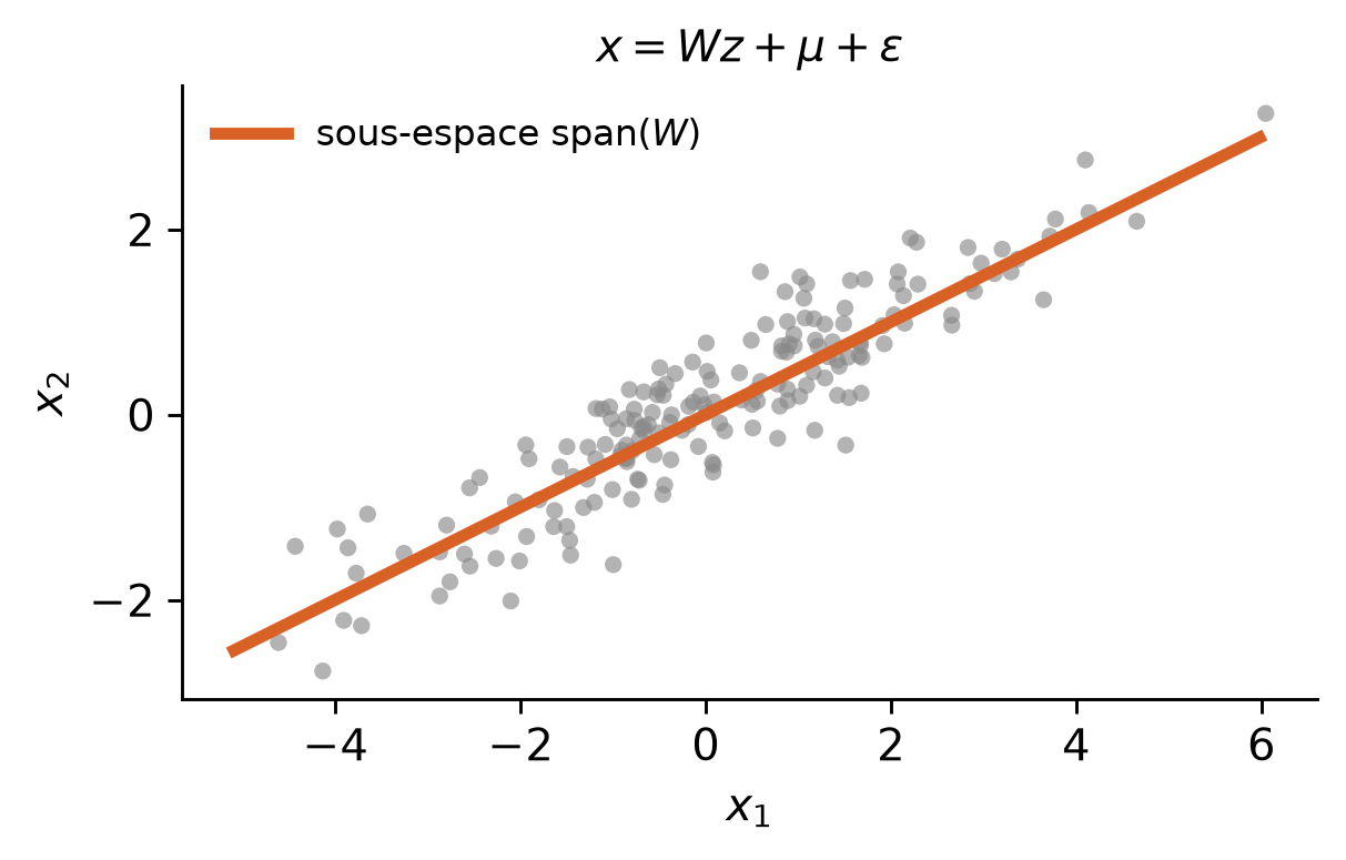
Modèle latent gaussien

Une structure linéaire de dimension \(q\), perturbée par un bruit isotrope.

\[ \mathbf{x}=\mathbf{\mu}+W\mathbf{z}+\mathbb{\varepsilon}, \]

\[ \begin{aligned} z &\sim \mathcal N(0,I_q), \\ x\mid z &\sim \mathcal N(\mu+Wz,\sigma^2I_p), \\ x &\sim \mathcal N(\mu,WW^\mathsf T+\sigma^2I_p). \end{aligned} \]

Figure 1

ACP probabiliste : Tipping et Bishop (1999).

Algorithme EM

E — moments conditionnels des coordonnées latentes.

M — paramètres \((\mu,W,\sigma^2)\) par vraisemblance complète espérée.

\[ \begin{aligned} Q(\theta\mid\theta^{(t)}) &=\mathbb E_{Z\mid X,\theta^{(t)}}[\log p(X,Z\mid\theta)],\\ \theta^{(t+1)}&=\arg\max_\theta Q(\theta\mid\theta^{(t)}). \end{aligned} \]

\(\sigma^2\to0\) : sous-espace estimé = sous-espace principal classique.

Réduire la dimension

Le problème

\(n\) individus, \(p\) variables quantitatives, souvent redondantes.

\(q<p\) coordonnées synthétiques.

Deux exigences : variance conservée, reconstruction fidèle.

Une ligne par individu, une colonne par variable.

\[ X= \begin{pmatrix} x_1^\mathsf T\\[-2pt] \vdots\\[-2pt] x_n^\mathsf T \end{pmatrix} \in\mathbb R^{n\times p}. \]

Le centre du nuage

Le barycentre des individus.

\[ \bar x=\frac1n\sum_{i=1}^n x_i, \qquad X_c=X-\mathbf 1_n\bar x^\mathsf T. \]

ACP = géométrie du nuage centré.

Deux géométries

Variables centrées

ACP de covariance

Unités conservées

Variables centrées-réduites

ACP de corrélation

Variances égales à 1

La standardisation change la question géométrique.

L’inertie totale

La dispersion quadratique autour du centre.

\[ I_T=\sum_{i=1}^n\lVert x_i-\bar x\rVert^2 =\lVert X_c\rVert_F^2. \]

Un sous-espace

\(F\subset\mathbb R^p\), dimension \(q\) ; \(P_F\) son projecteur orthogonal.

\[ \widehat x_i=\bar x+P_F(x_i-\bar x), \qquad r_i=(I_p-P_F)(x_i-\bar x). \]

Le triangle rectangle

Pour chaque individu : inertie = projection + résidu.
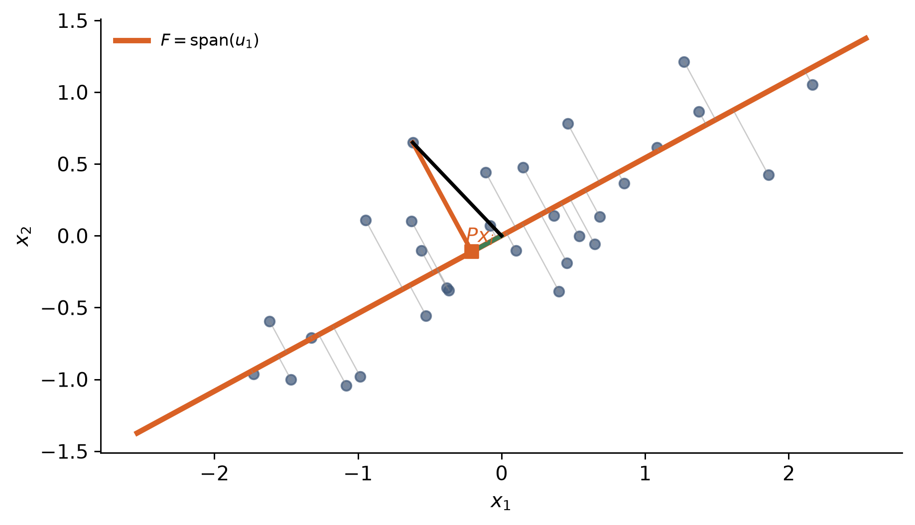
Figure 2

Pythagore, pour le nuage

La somme des identités individuelles.

\[ \underbrace{I_T}_{\text{inertie totale}} = \underbrace{\sum_i\lVert P_F(x_i-\bar x)\rVert^2}_{I_{\mathrm{proj}}(F)} + \underbrace{\sum_i\lVert(I_p-P_F)(x_i-\bar x)\rVert^2}_{I_{\mathrm{res}}(F)}. \]

\(I_T=I_{\mathrm{proj}}+I_{\mathrm{res}}\) — égalité exacte.

Deux critères, un optimum

À dimension \(q\) fixée, même sous-espace optimal.

\[ \arg\max_{\dim(F)=q} I_{\mathrm{proj}}(F) = \arg\min_{\dim(F)=q} I_{\mathrm{res}}(F). \]

La solution spectrale

Matrice de covariance

Convention population, cohérente avec l’inertie.

\[ S=\frac1nX_c^\mathsf TX_c, \qquad S=S^\mathsf T\succeq0. \]

Une direction unitaire

Coordonnées projetées : \(c=X_cu\).

Variance portée par l’axe \(u\).

\[ \frac1n\lVert c\rVert^2 =\frac1n\lVert X_cu\rVert^2 =u^\mathsf TSu, \qquad \lVert u\rVert=1. \]

Premier axe principal

Tout maximiseur est un vecteur propre associé à \(\lambda_1\).

\[ \max_{\lVert u\rVert=1}u^\mathsf TSu=\lambda_1, \qquad Su_1=\lambda_1u_1, \qquad \lambda_1\geq\lambda_2\geq\cdots\geq\lambda_p\geq0. \]

Premier axe : démonstration

Théorème spectral : \(S=\sum_j\lambda_ju_ju_j^\mathsf T\), base \((u_j)\) orthonormée.

\[ \begin{aligned} u&=\sum_ja_ju_j,\qquad \sum_ja_j^2=1,\\ u^\mathsf TSu&=\sum_j\lambda_ja_j^2\leq\lambda_1\sum_ja_j^2=\lambda_1. \end{aligned} \]

  • Égalité en \(u=u_1\) : maximum atteint.
  • Égalité \(\iff\) \(a_j=0\) dès que \(\lambda_j<\lambda_1\) : \(u\) dans l’espace propre de \(\lambda_1\), donc \(Su=\lambda_1u\).
  • Positivité : \(\lambda_j=u_j^\mathsf TSu_j=\frac1n\lVert X_cu_j\rVert^2\geq0\).

Sous-espace principal

Les \(q\) premiers axes engendrent le meilleur sous-espace.

\[ F_q=\operatorname{span}(u_1,\ldots,u_q), \qquad P_q=U_qU_q^\mathsf T. \]

Sous-espace principal : démonstration

\(P\) projecteur sur \(F\), \(h_j=\lVert Pu_j\rVert^2\in[0,1]\) : \(\sum_jh_j=\operatorname{tr}P=q\) et \(I_{\mathrm{proj}}(F)=n\operatorname{tr}(PS)=n\sum_j\lambda_jh_j\).

\[ \begin{aligned} \tfrac1nI_{\mathrm{proj}}(F)-\sum_{j\leq q}\lambda_j &=\sum_{j\leq q}\lambda_j(h_j-1)+\sum_{j>q}\lambda_jh_j\\ &\leq\lambda_q\Big(\sum_jh_j-q\Big)=0. \end{aligned} \]

  • Égalité pour \(F_q\) (\(h_j=1\) si \(j\leq q\), \(0\) sinon) ; unique si \(\lambda_q>\lambda_{q+1}\).
  • \(q=1\) : \(h_j=a_j^2\), preuve du premier axe.

Composantes principales

Scores des individus dans la nouvelle base ; covariances nulles.

\[ C=X_cU, \qquad \frac1nC^\mathsf TC=\Lambda. \]

Formule de reconstitution

Reconstruction de rang \(q\).

\[ \widehat X_q=C_qU_q^\mathsf T =X_cU_qU_q^\mathsf T =X_cP_q. \]

Théorème d’Eckart–Young

\(\widehat X_q\) est la meilleure approximation de rang au plus \(q\).

\[ \widehat X_q\in \arg\min_{\operatorname{rang}(A)\leq q}\lVert X_c-A\rVert_F^2, \qquad \lVert X_c-\widehat X_q\rVert_F^2=n\sum_{j>q}\lambda_j. \]

Inerties spectrales

Chaque axe porte \(n\lambda_j\) unités d’inertie.

\[ \begin{aligned} I_T&=n\sum_{j=1}^p\lambda_j=n\operatorname{tr}(S),\\ I_{\mathrm{proj}}(F_q)&=n\sum_{j=1}^q\lambda_j,\\ I_{\mathrm{res}}(F_q)&=n\sum_{j=q+1}^p\lambda_j. \end{aligned} \]

Dimension \(q\)

Taux d’inertie expliquée.

\[ \rho_q=\frac{I_{\mathrm{proj}}(F_q)}{I_T} =\frac{\sum_{j=1}^q\lambda_j}{\sum_{j=1}^p\lambda_j}. \]

Seuil, coude, interprétabilité — trois critères, aucun automatisme.

Iris sans étiquette

Standardisation

150 fleurs, quatre mesures en centimètres, quatre variances unitaires.

species retirée avant tout calcul.

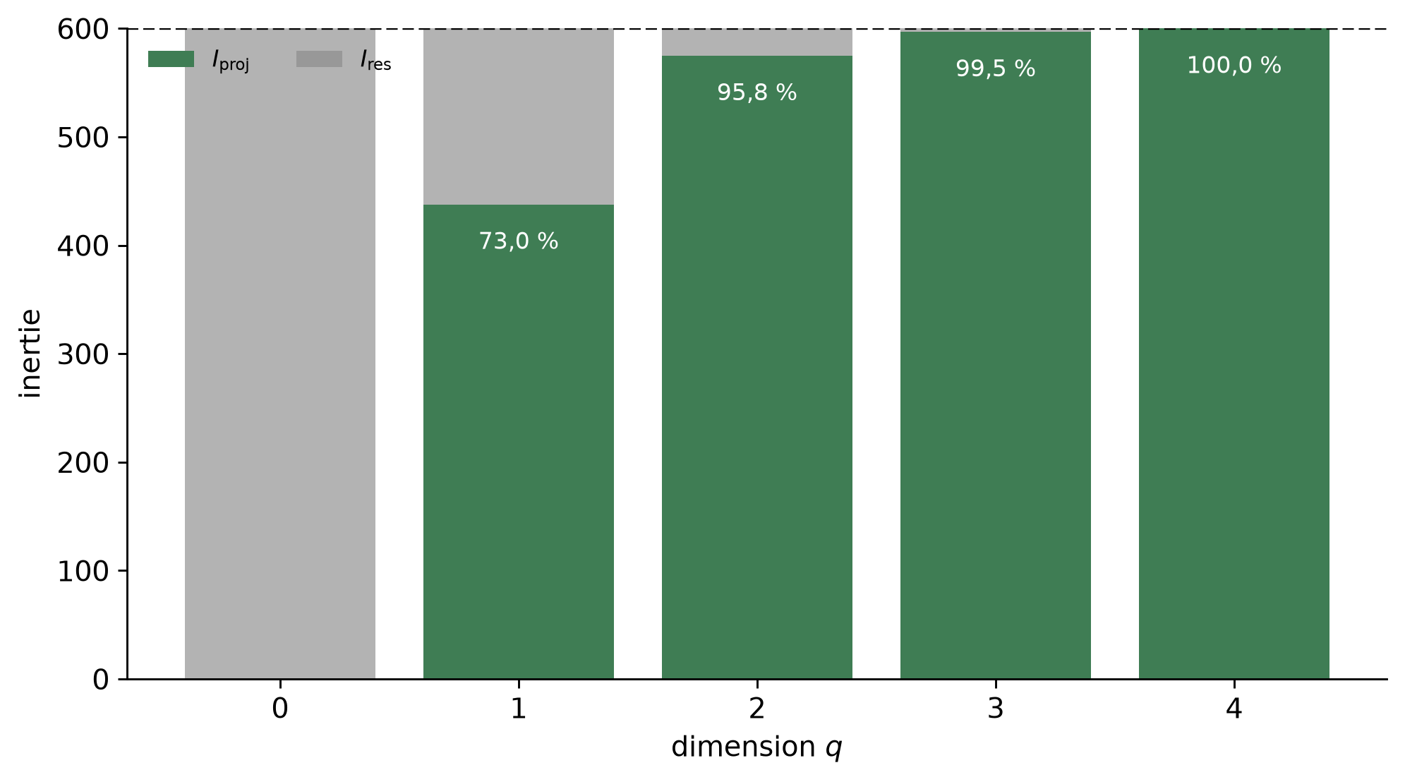
\[ z_{ij}=\frac{x_{ij}-\bar x_j}{s_j}, \qquad \operatorname{tr}(S)=4, \qquad I_T=np=600. \]

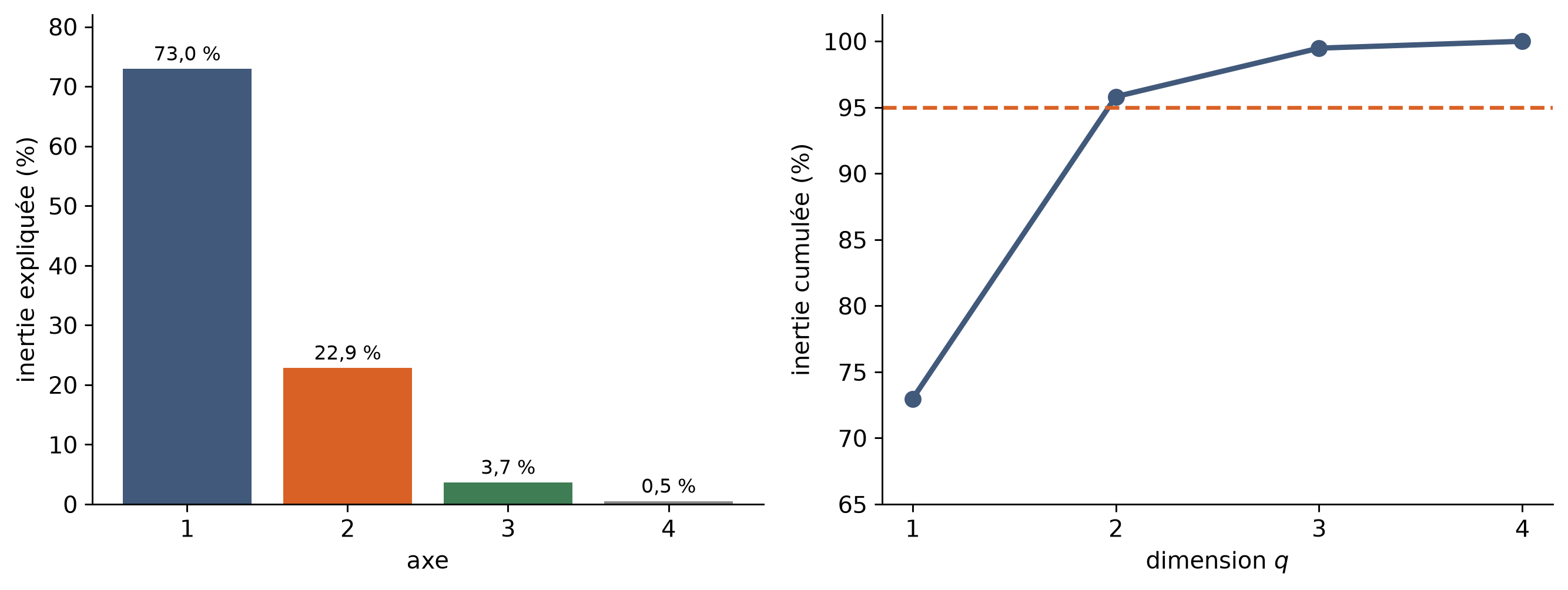
Le spectre

Figure 3

Deux axes : \(95{,}8\,\%\) de l’inertie.

Le plan principal
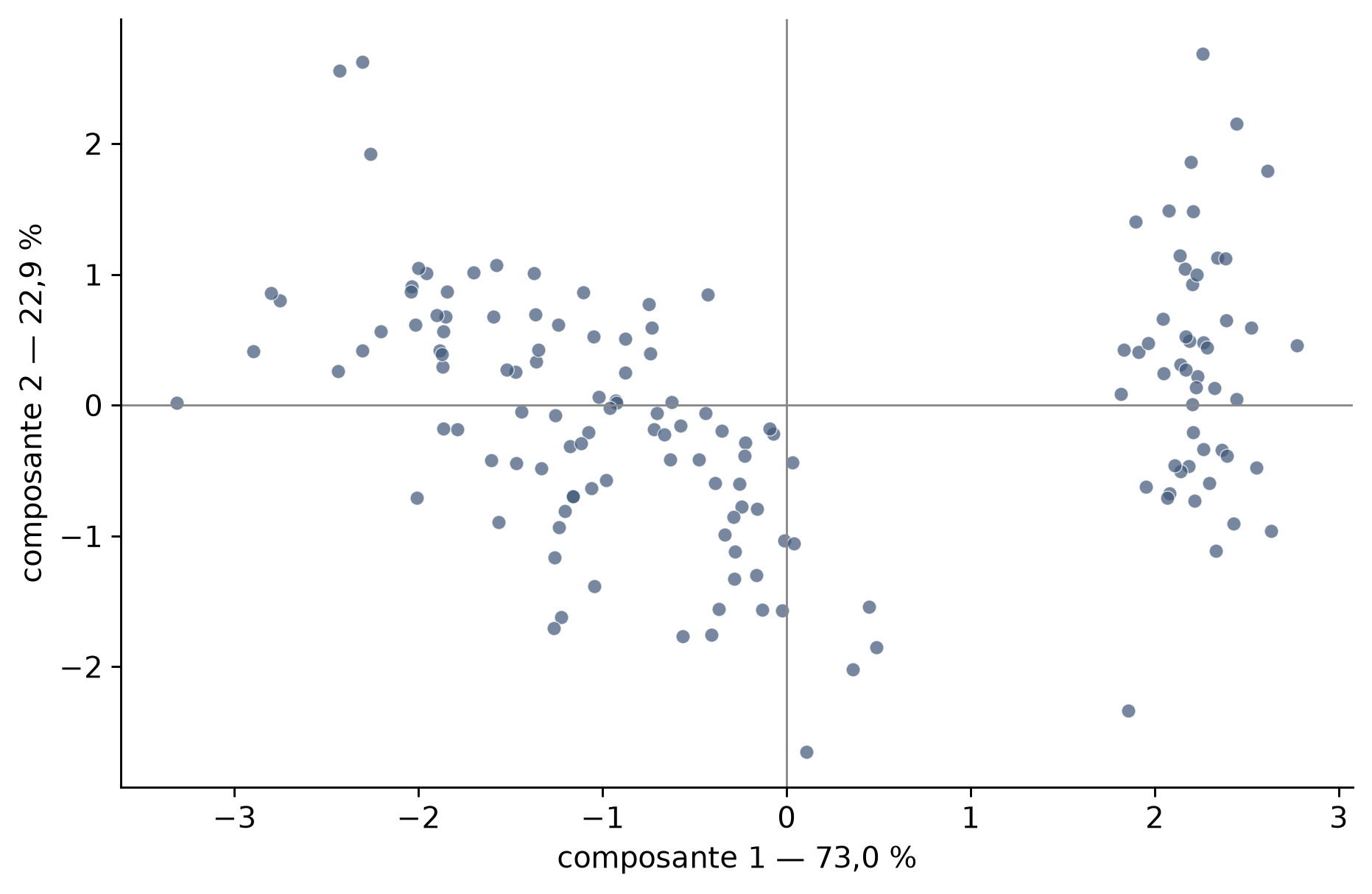
Figure 4

Aucune classe dans la construction.

Lecture a posteriori
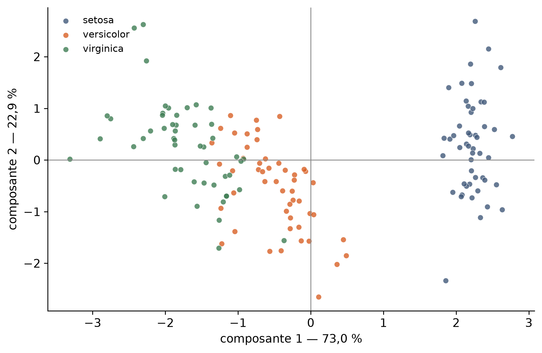
Figure 5

Les espèces colorent un résultat déjà calculé.

Corrélation variable–composante

Variable standardisée \(z_j\) (colonne de \(Z\)), composante \(c_k=Zu_k\), \(S=\frac1nZ^\mathsf TZ\) ; \(\widehat{\operatorname{cor}}\) : corrélation empirique.

\[ \begin{aligned} \widehat{\operatorname{cov}}(z_j,c_k)&=\tfrac1nz_j^\mathsf TZu_k=(Su_k)_j=\lambda_ku_{jk},\\ \widehat{\operatorname{var}}(z_j)&=1,\qquad\widehat{\operatorname{var}}(c_k)=u_k^\mathsf TSu_k=\lambda_k,\\ \widehat{\operatorname{cor}}(z_j,c_k)&=\frac{\lambda_ku_{jk}}{\sqrt{1\cdot\lambda_k}}=\sqrt{\lambda_k}\,u_{jk}. \end{aligned} \]

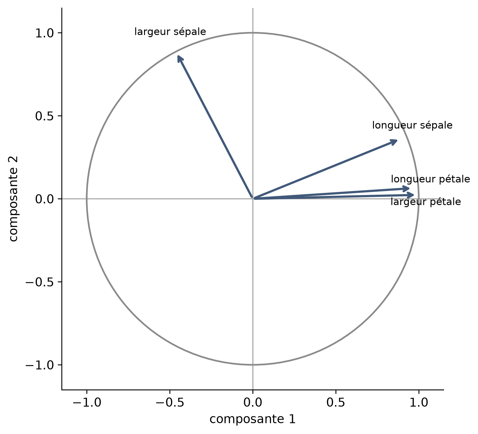
Proximité, opposition, orthogonalité — lecture par angles.

Cercle des corrélations

Figure 6

Qualité d’un individu

Part de sa distance au centre visible dans le premier plan.

\[ \cos^2(i,F_q) =\frac{\lVert P_q(x_i-\bar x)\rVert^2}{\lVert x_i-\bar x\rVert^2} =\frac{\sum_{j=1}^q c_{ij}^2}{\lVert x_i-\bar x\rVert^2}. \]

Contribution d’un individu

Part de l’inertie de l’axe \(j\) due à l’individu \(i\).

\[ \operatorname{CTR}(i,j)=\frac{c_{ij}^2}{n\lambda_j}, \qquad \sum_{i=1}^n\operatorname{CTR}(i,j)=1. \]

Qualité : représentation de \(i\). Contribution : influence de \(i\) sur l’axe.

Reconstruction par rang

Figure 7

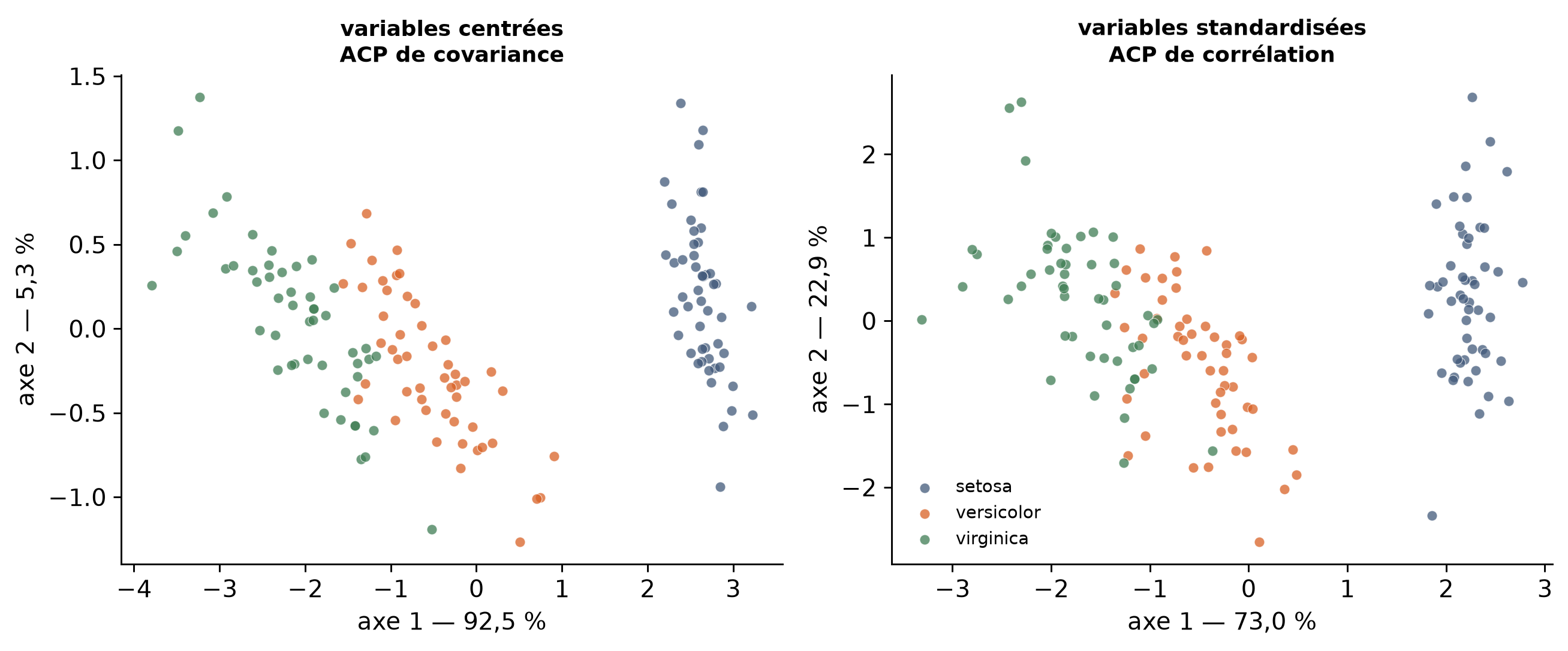
Le choix des unités

Figure 8

Covariance : variabilité physique. Corrélation : variabilité relative.

Deux théorèmes de la variance

Pythagore pour \(k\)-means

Pour \(x_i\) dans le groupe \(G_k\), centre \(\mu_k\), centre global \(\mu\).

\[ \begin{aligned} x_i-\mu&=(x_i-\mu_k)+(\mu_k-\mu),\\ \sum_{i\in G_k}(x_i-\mu_k)&=0. \end{aligned} \]

Le terme croisé disparaît après sommation dans chaque groupe.

Inertie intra + inter

Théorème de Huygens, analogue multivarié de la variance totale.

\[ \underbrace{\sum_i\lVert x_i-\mu\rVert^2}_{I_T} = \underbrace{\sum_k\sum_{i\in G_k}\lVert x_i-\mu_k\rVert^2}_{I_W} + \underbrace{\sum_kn_k\lVert\mu_k-\mu\rVert^2}_{I_B}. \]

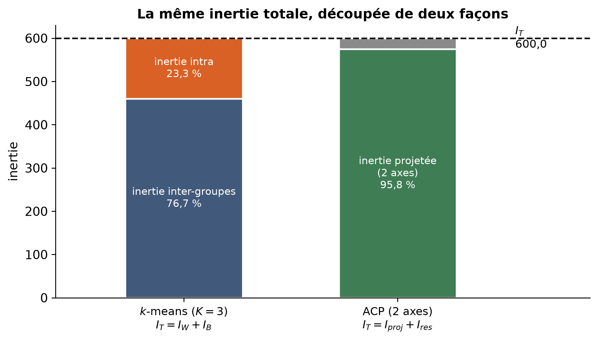
Deux partitions de \(I_T\)

Figure 9

Deux questions

ACP

Sous-espace linéaire

\(I_{\mathrm{res}}\) minimal

Compression, visualisation

\(k\)-means

Partition discrète

\(I_W\) minimal

Groupes, quantification

Même inertie totale. Orthogonalité individuelle pour l’ACP ; centrage par groupe pour \(k\)-means.

En bref

  1. ACP : meilleure projection orthogonale de rang \(q\).
  2. Spectre : inertie projetée axe par axe.
  3. Pythagore : \(I_T=I_{\mathrm{proj}}+I_{\mathrm{res}}\).
  4. \(k\)-means : \(I_T=I_W+I_B\).
  5. Modèle gaussien latent : même sous-espace, lecture probabiliste et EM.