Causal discovery with non-Gaussian noise: LiNGAM and OT-LiNGAM

Lecture 6 — Causality and Graphical Models

Christophe Ambroise

M2 Data Science — Université d’Évry

Prior knowledge

Lectures 4 and 5

  • SCM \(V_j := f_j(V_{pa(j)}, U_j)\); intervention = graph surgery
  • Backdoor adjustment; instrument and Wald ratio
  • Structure learning: constraint-based (PC), score-based (BIC, GES)
  • PC output: CPDAG, Markov equivalence class
  • Gaussian linear SEM: direction of \(X_1 - X_2\) not identifiable
  • SHD: additions + deletions + reversals

Beyond Markov equivalence: LiNGAM

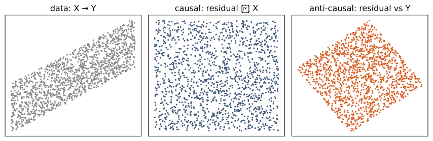
Two variables, one direction?

  • Both residuals uncorrelated with the regressor
  • Only the causal one independent: non-Gaussianity breaks the symmetry

Linear non-Gaussian acyclic model

In LiNGAM, the data follow a linear SEM on a DAG, with mutually independent noises of which at most one is Gaussian.

\[ X = B X + \varepsilon, \qquad B \text{ acyclic (strictly lower triangular up to permutation)}, \qquad \varepsilon_1, \dots, \varepsilon_d \text{ independent} \]

Identifiability (Shimizu et al., 2006) Under these assumptions, \(B\) and the causal order are identifiable from the distribution of \(X\) alone.

Darmois–Skitovich theorem

If two linear combinations of independent variables are independent, every variable appearing in both is Gaussian.

\[ \varepsilon_j \text{ independent},\ \ \textstyle\sum_j a_j \varepsilon_j \perp \sum_j b_j \varepsilon_j \;\Longrightarrow\; \forall j : a_j b_j \neq 0 \Rightarrow \varepsilon_j \text{ Gaussian} \]

  • Anti-causal residual \(X - \hat b Y\) and \(Y\): both mix \(\varepsilon_X\)
  • Non-Gaussian \(\varepsilon_X\) → dependence → wrong direction detected

DirectLiNGAM

\(X_j\) is exogenous (a source) if and only if every other variable, regressed on \(X_j\), leaves a residual independent of \(X_j\).

\[ X_j \text{ source} \iff \forall\, i \neq j : \quad X_i - \frac{\operatorname{Cov}(X_i, X_j)}{\operatorname{Var} X_j} X_j \;\perp\; X_j \]

  1. Most independent candidate → next variable of the order
  2. Its effect regressed out of all remaining variables
  3. Repeat; then \(B\) by adaptive lasso along the order

Shimizu et al. (2011), JMLR. Python package lingam.

DirectLiNGAM in practice

import numpy as np, lingam
rng = np.random.default_rng(1); n = 2000
e = rng.laplace(size=(n, 4))                     # non-Gaussian noises
x0 = e[:, 0]
x2 = 0.8 * x0 + e[:, 2]
x1 = -0.7 * x2 + e[:, 1]
x3 = 0.5 * x0 + 0.6 * x1 + e[:, 3]
X = np.c_[x0, x1, x2, x3]
model = lingam.DirectLiNGAM().fit(X)
print("order:", [int(i) for i in model.causal_order_])
print(np.round(model.adjacency_matrix_, 2))      # B[j, k] : effect k -> j
order: [0, 2, 1, 3]
[[ 0.    0.    0.    0.  ]
 [ 0.    0.   -0.69  0.  ]
 [ 0.79  0.    0.    0.  ]
 [ 0.51  0.6   0.    0.  ]]

OT-LiNGAM: non-Gaussianity by optimal transport

Measuring non-Gaussianity

  • Classical contrasts: kurtosis, negentropy approximations, likelihood surrogates
  • Choice of a nonlinearity or moment order → method tuned to source shape
  • Wanted: one criterion, no tuning, only finite second moments

Laplante, Ambroise & Humbert, Contrast-free ICA and causal inference via Wasserstein distances to the Gaussian, preprint. Package otlingam.

2-Wasserstein distance

The squared 2-Wasserstein distance is the smallest mean squared displacement among all couplings of the two distributions.

\[ \mathcal W_2(\mu, \nu)^2 = \inf_{X \sim \mu,\ Y \sim \nu} \mathbb E\big[(X - Y)^2\big] \overset{\text{dim } 1}{=} \int_0^1 \big(F_\mu^{-1}(u) - F_\nu^{-1}(u)\big)^2\, du \]

  • Dimension 1: optimal coupling = matching of quantiles
  • Non-Gaussianity of \(X\): \(\;\mathcal W_2\big(\operatorname{std}(X), \mathcal N(0, 1)\big)^2\), zero iff \(X\) Gaussian

Exact empirical computation

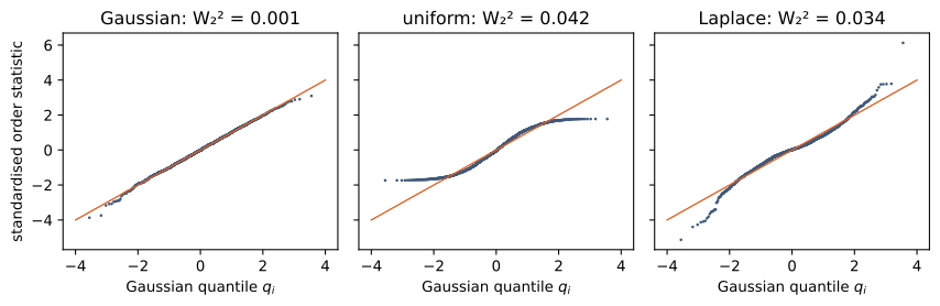
For a sample \(x^{(1:n)} \leq \dots \leq x^{(n:n)}\), the distance to \(\mathcal N(0, 1)\) is a sum of squares between order statistics and Gaussian quantile averages.

\[ \mathcal W_2\big(\mu_n, \mathcal N(0, 1)\big)^2 = \frac1n \sum_{i=1}^{n} \big(x^{(i:n)} - q_i\big)^2 + c_n, \qquad q_i = n\big(\phi(z_{i-1}) - \phi(z_i)\big),\ \ z_i = \Phi^{-1}(i/n) \]

  • \(c_n = 1 - \frac1n \sum_i q_i^2\): constant
  • Cost \(O(n \log n)\): one sort

Non-Gaussianity of three distributions

Mixtures are closer to the Gaussian

Under independence and standardisation, any non-trivial normalised mixture of sources is strictly closer to the Gaussian than the corresponding weighted average of the sources’ distances.

\[ \|\alpha\|_2 = 1,\ \#\{j : \alpha_j \neq 0\} > 1 \;\Longrightarrow\; \mathcal W_2\Big(\sum_j \alpha_j S_j, \mathcal N(0, 1)\Big)^2 < \sum_j \alpha_j^2\, \mathcal W_2\big(S_j, \mathcal N(0, 1)\big)^2 \]

Assumptions: \(S_j\) independent, centred, unit variance, at most one Gaussian.

Wasserstein order objective

For a candidate order \(\sigma\), regress each variable on its predecessors and score the non-Gaussianity of the standardised residuals.

\[ G(\sigma) = \sum_{j=1}^{d} \mathcal W_2\Big(\operatorname{std}\big(R_j(\sigma)\big), \mathcal N(0, 1)\Big)^2, \qquad R_j(\sigma) = X_j - \operatorname{proj}_{\operatorname{span}\{X_k : k \text{ before } j\}} X_j \]

  • Causal order: residuals = structural noises \(\varepsilon_j\)
  • Wrong order: some residual mixes several noises → closer to Gaussian

Identification of causal orders

Theorem (Laplante, Ambroise & Humbert) Under independent, non-degenerate noises with at most one Gaussian, the maximisers of \(G\) are exactly the causal orders of the model.

\[ \arg\max_{\sigma \in \mathfrak S_d} G(\sigma) = \mathcal I^\star = \big\{\sigma : \Pi^\sigma B (\Pi^\sigma)^\top \text{ strictly lower triangular}\big\} \]

Key steps: \(\operatorname{std}(R(\sigma)) = Q^\sigma \operatorname{std}(\varepsilon)\) with \(Q^\sigma\) orthogonal; strict subadditivity; \(Q^\sigma\) signed permutation \(\Rightarrow\) \(\sigma\) causal.

Consistency

  • Empirical objective \(\hat G_n\): OLS residuals + exact \(\mathcal W_2\)
  • Uniform convergence: \(\max_\sigma |\hat G_n(\sigma) - G(\sigma)| \to 0\) a.s., finite second moments only
  • Margin \(\Gamma = \max G - \max_{\sigma \notin \mathcal I^\star} G > 0\)

\[ \mathbb P\big(\hat\sigma_n \notin \mathcal I^\star\big) \leq \mathbb P\Big(\max_\sigma |\hat G_n(\sigma) - G(\sigma)| \geq \Gamma / 2\Big) \to 0 \]

  • Sub-Gaussian data: rate \(d^{5/4} n^{-1/4}\) up to log factors

Exhaustive solver: dynamic programming

Decomposable score → recursion on subsets \(U\), \(H(U)\) = best score of an order of \(U\):

\[ H(U) = \max_{u \in U} \Big\{ H(U \setminus \{u\}) + \hat g_u(U \setminus \{u\}) \Big\}, \qquad H(\emptyset) = 0 \]

  • \(\hat g_u(P)\): non-Gaussianity of the residual of \(X_u\) on \(X_P\)
  • Backtracking of the stored sinks → order
  • \(d\,2^{d-1}\) local scores instead of \(d!\) orders; exact optimum up to \(d \approx 30\)

Greedy solver and full pipeline

Greedy OT-LiNGAM: most non-Gaussian standardised residual → next source; its effect regressed out; repeat. Cost \(O(d^2 n \log n)\).

Solver Cost Global optimum
Exhaustive OT-LiNGAM \(O\big(d 2^d (n d^2 + n \log n)\big)\) yes
Greedy OT-LiNGAM \(O(d^2 n \log n)\) no
OT-ICA-LiNGAM \(O(n d^2 + d n \log n)\) / iteration no

Order known → \(B\) by adaptive lasso along the order.

Evaluation: disorder of an order

Number of true edges reversed by the estimated order:

\[ \operatorname{dis}(\hat\sigma) = \#\big\{(k, j) : B_{jk} \neq 0,\ \hat\sigma^{-1}(k) > \hat\sigma^{-1}(j)\big\} \]

  • \(\operatorname{dis}(\hat\sigma) = 0 \iff \hat\sigma\) causal order
  • Simulations of the paper (ER and scale-free graphs, Laplace or Student noises): exhaustive OT-LiNGAM close to zero disorder, robust when some noises approach Gaussianity
  • Continuous methods (DAGMA): degraded under heteroscedastic noises

OT-LiNGAM in practice

import numpy as np
from otlingam import ExhaustiveOTLiNGAM, GreedyOTLiNGAM
from otlingam.utils import disorder
rng = np.random.default_rng(1); n = 2000
e = rng.laplace(size=(n, 4))
x0 = e[:, 0]; x2 = 0.8 * x0 + e[:, 2]
x1 = -0.7 * x2 + e[:, 1]; x3 = 0.5 * x0 + 0.6 * x1 + e[:, 3]
X = np.c_[x0, x1, x2, x3]
B_true = np.zeros((4, 4)); B_true[2, 0], B_true[1, 2], B_true[3, 0], B_true[3, 1] = .8, -.7, .5, .6
for M in (ExhaustiveOTLiNGAM(), GreedyOTLiNGAM()):
    M.fit(X)
    print(type(M).__name__, [int(i) for i in M.causal_order_], "disorder:", disorder(B_true, M.causal_order_))
ExhaustiveOTLiNGAM [0, 2, 1, 3] disorder: 0
GreedyOTLiNGAM [0, 2, 1, 3] disorder: 0

LiNGAM analysis in practice

Non-Gaussianity check

from scipy import stats
print("excess kurtosis:", np.round(stats.kurtosis(X), 2))
print("Shapiro p-values:", [f"{stats.shapiro(c).pvalue:.1e}" for c in X.T])
excess kurtosis: [2.72 0.99 1.57 1.21]
Shapiro p-values: ['4.8e-21', '5.6e-09', '2.0e-15', '2.5e-10']
  • Kurtosis far from 0, tiny Shapiro p-values: non-Gaussian variables
  • Near-Gaussian variables: directions unreliable
  • Discrete or binary variables: LiNGAM only an approximation

Bootstrap stability of edges

model = lingam.DirectLiNGAM().fit(X)
boot = lingam.DirectLiNGAM().bootstrap(X, n_sampling=100)  # separate instance: refitted in place
P = boot.get_probabilities(min_causal_effect=0.05)  # P[j, k]: frequency of edge k -> j
print(np.round(P, 2))
[[0.   0.   0.   0.  ]
 [0.01 0.   1.   0.  ]
 [1.   0.   0.   0.  ]
 [1.   1.   0.02 0.  ]]
  • One fit = one estimate; bootstrap = frequency of each edge over resamples
  • Edges reported with their frequency

Independence of residuals

print(np.round(model.get_error_independence_p_values(X), 2))
rng = np.random.default_rng(1); h = rng.laplace(size=n)   # h: hidden common cause
a = h + rng.laplace(size=n); b = 0.5 * a + h + rng.laplace(size=n)
D = np.c_[a, b]; m = lingam.DirectLiNGAM().fit(D)
pv = m.get_error_independence_p_values(D)[0, 1]
print(f"a -> b: {m.adjacency_matrix_[1, 0]:.2f}, p-value {pv:.0e}")
[[0.   0.82 0.12 0.17]
 [0.82 0.   0.35 0.74]
 [0.12 0.35 0.   0.67]
 [0.17 0.74 0.67 0.  ]]
a -> b: 0.97, p-value 3e-06
  • Model assumption: independent noises → residuals pairwise independent
  • Small p-value: hidden confounder, non-linearity or feedback
  • Hidden \(h\): effect \(0.97\) instead of \(0.5\), residuals clearly dependent

Prior knowledge

pk = lingam.utils.make_prior_knowledge(4, exogenous_variables=[0], sink_variables=[3])
print(pk)                          # pk[j, k]: 1 path k -> j, 0 no path, -1 unknown
print([int(i) for i in lingam.DirectLiNGAM(prior_knowledge=pk).fit(X).causal_order_])
[[-1  0  0  0]
 [-1 -1 -1  0]
 [-1 -1 -1  0]
 [-1 -1 -1 -1]]
[0, 2, 1, 3]
  • Exogenous variables: genotype, treatment, time
  • Sinks: final phenotype, outcome
  • Fewer orders to search, fewer errors

Total causal effect

The total effect of \(X_k\) on \(X_j\) sums the contributions of all directed paths from \(X_k\) to \(X_j\): the change of \(X_j\) under an intervention \(do(X_k = x + 1)\) instead of \(do(X_k = x)\).

print(f"x0 -> x3: {model.estimate_total_effect(X, 0, 3):.2f}")
x0 -> x3: 0.18
  • True value: direct \(0.5\) + path \(x_0 \to x_2 \to x_1 \to x_3\): \(0.8 \times (-0.7) \times 0.6\) → \(0.164\)
  • Bootstrap version: boot.get_total_causal_effects()

Estimators and report

Estimator Package Use
DirectLiNGAM lingam bootstrap, prior knowledge, tests
ExhaustiveOTLiNGAM otlingam exact search, few variables
GreedyOTLiNGAM otlingam many variables

Report of a LiNGAM analysis Non-Gaussianity; orders from two estimators; bootstrap frequencies of the edges; residual tests; prior knowledge; total effects.

Case study: chloroplast RNA maturation

Biological context

  • Chloroplast transcripts of Arabidopsis thaliana: genes ndhB, ndhD
  • Post-transcriptional maturation: C-to-U editing at specific sites, intron splicing
  • Nanopore long reads: one read = one full-length RNA molecule
  • Each read: snapshot of one molecule at some stage of its maturation

Data: Guilcher et al. (2021), Int. J. Mol. Sci. 22, 11297.

Data: one binary vector per read

  ed1   ed2   ed3   ed4  ed5
False False False  True    ·
 True False     ·     ·    ·
False False False False    ·
False  True False  True    ·
 True False False  True True
False  True  True  True    ·
Gene Reads Events Complete reads
ndhB 1 899 12 editing sites + intron splicing 117
ndhD 7 574 5 editing sites 930

True: event observed; False: not observed; Err: sequencing error; empty: not covered.

Question: chronology of maturation events

  • Order in which sites are edited and the intron spliced
  • Chronology as a causal order of the event variables
  • Snapshot data only: no time stamps

Open problem Can a causal order learned from snapshots of molecules reveal the maturation chronology?

Methodological difficulties

  • Binary variables: linear non-Gaussian model only an approximation
  • Missing blocks: reads truncated, contiguous sites unobserved
  • Errors (Err): measurement noise on some sites
  • Rare events (sites edited in < 10 % of reads)
  • Validation: no ground-truth chronology