
Structure learning: scores and conditional independence tests

Lecture 5 — Causality and Graphical Models

Christophe Ambroise

M2 Data Science — Université d’Évry

Prior knowledge

Lectures 3 and 4

  • Gaussian graphical model: support of \(K = \Sigma^{-1}\); graphical lasso
  • Moral graph: support of \(K\) for a Gaussian DAG
  • SCM: \(V_j := f_j(V_{pa(j)}, U_j)\); \(do(X = x)\) = graph surgery
  • Truncated factorisation; backdoor formula \(P(y \mid do(x)) = \sum_z P(y \mid x, z) P(z)\)
  • Instrument, Mendelian randomisation: Wald ratio \(\beta_{ZY} / \beta_{ZX}\)

Structure learning

Structure learning: goals and obstacle

  • Knowledge discovery: graph topology (gene networks, signalling pathways)
  • Density estimation: fully specified model
  • Obstacle: super-exponential number of DAGs
\(p\) 2 3 4 5 10
DAGs 3 25 543 29 281 \(4.2 \times 10^{18}\)

Robinson (1973). Structure learning of DAGs: NP-hard (Chickering, 1996).

Three families of methods

Family Principle Output
constraint-based conditional independence tests CPDAG (PC, FCI)
score-based score optimisation over graphs DAG or CPDAG (hill climbing, GES)
functional restricted SCM class DAG (LiNGAM, ANM)

Trees: the Chow–Liu algorithm

Relevance networks

  • Edge \(i - j\) if mutual information \(I(X_i; X_j) > \alpha\)
  • Gaussian case: \(I(X_i; X_j) = -\tfrac12 \log(1 - \rho_{ij}^2)\) → thresholded correlations
  • Problem: dense graphs, marginal not conditional dependences

Tree-structured distributions

Undirected tree \(T\), root choice irrelevant:

\[ p(x \mid T) = \prod_{t \in V} p(x_t) \prod_{(s, t) \in E(T)} \frac{p(x_s, x_t)}{p(x_s)\, p(x_t)} \]

Maximised log-likelihood, empirical frequencies \(\hat p\):

\[ \frac1N \log p(\mathcal D \mid \hat\theta, T) = -\sum_{t} \hat H(X_t) + \sum_{(s,t) \in E(T)} \hat I(X_s; X_t) \]

Chow–Liu theorem

The maximum likelihood tree is the maximum weight spanning tree of the complete graph weighted by empirical mutual informations.

\[ \hat T = \arg\max_{T \text{ spanning tree}} \sum_{(s, t) \in E(T)} \hat I(X_s; X_t) \]

  • Kruskal or Prim: \(O(p^2 \log p)\)
  • Exact optimum in polynomial time, unlike general DAGs

Chow & Liu (1968), IEEE Trans. Inf. Theory.

Kruskal algorithm

  1. Edges sorted by decreasing weight \(\hat I(X_s; X_t)\)
  2. \(T \leftarrow \emptyset\)
  3. Next edge added iff no cycle created in \(T\)
  4. Stop at \(p - 1\) edges

Extensions: tree-augmented naive Bayes (TAN), mixtures of trees.

Score-based learning

Decomposable scores

A score is decomposable when it is a sum of local terms, one per node and its parent set.

\[ \operatorname{score}(G; \mathcal D) = \sum_{t \in V} s\big(X_t, X_{pa_G(t)}; \mathcal D\big) \]

  • Local change (one edge) → one or two terms recomputed
  • Same decomposition as the likelihood

BIC score

\[ \operatorname{BIC}(G) = \sum_{t \in V} \Big[\, \ell_t\big(\hat\theta_t\big) - \frac{\log N}{2}\, d_t \Big] \]

  • \(\ell_t\): maximised log-likelihood of node \(t\) given its parents
  • \(d_t\): number of free parameters of the CPD of \(t\)
  • Penalty → sparse graphs; consistent model selection

Bayesian score (BDe)

Dirichlet prior on each CPT → closed-form marginal likelihood:

\[ p(\mathcal D \mid G) = \prod_{t} \prod_{c = 1}^{C_t} \frac{B(N_{tc\cdot} + \alpha_{tc\cdot})}{B(\alpha_{tc\cdot})} \]

  • BDe: \(\alpha_{tck} = \alpha\, p_0(x_t = k, x_{pa(t)} = c)\)
  • Score equivalence: same score for Markov-equivalent DAGs

Heckerman, Geiger & Chickering (1995); Geiger & Heckerman (1997).

Search strategies

  • Hill climbing over DAGs: add, delete or reverse one edge; best improvement; local optimum
  • Restarts, tabu list against local optima
  • GES (Chickering, 2002): greedy search over equivalence classes, forward then backward phase
  • GES + consistent score: true CPDAG in the large-sample limit

Constraint-based learning: the PC algorithm

Assumptions

  • Causal Markov: d-separation ⇒ independence
  • Faithfulness: independence ⇒ d-separation
  • Causal sufficiency: no unobserved common cause
  • Reliable conditional independence tests

Key fact \(i\) and \(j\) non-adjacent in \(G\) iff some set \(S\) makes them independent: \(X_i \perp X_j \mid X_S\).

Conditional independence tests

  • Gaussian: partial correlation, Fisher \(z\) transform

\[ z = \tfrac12 \log\frac{1 + \hat\rho_{ij \cdot S}}{1 - \hat\rho_{ij \cdot S}}\, \sqrt{N - |S| - 3} \;\approx\; \mathcal N(0, 1) \text{ under } H_0 \]

  • Discrete: \(\chi^2\) or \(G^2\) test on contingency tables
  • Non-linear: kernel tests (KCI)
  • Level \(\alpha\): sparsity knob

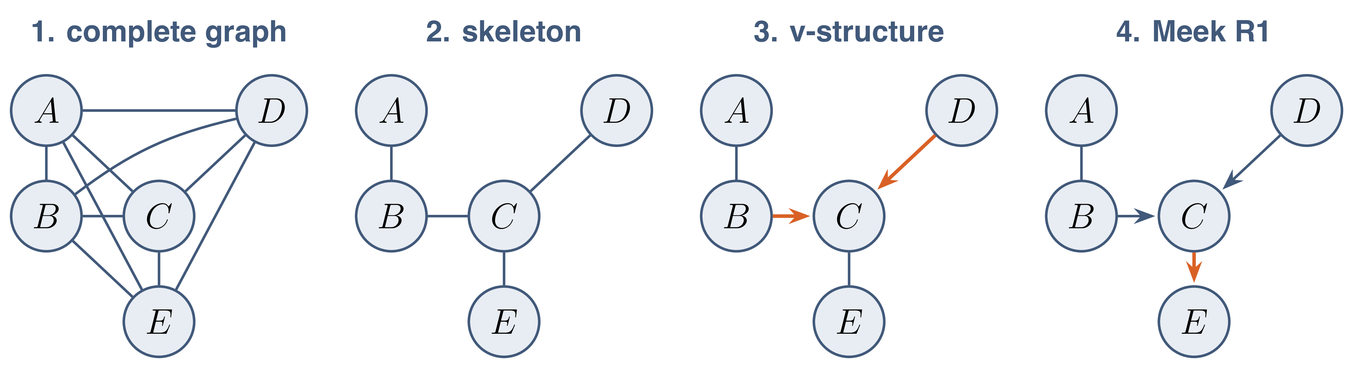
PC step 1: skeleton

  1. Start: complete undirected graph
  2. For \(\ell = 0, 1, 2, \dots\): for each edge \(i - j\), test \(X_i \perp X_j \mid X_S\) for \(S \subseteq adj(i) \setminus \{j\}\), \(|S| = \ell\)
  3. Independence accepted → edge removed, \(\operatorname{sepset}(i, j) = S\)
  4. Stop when no node has more than \(\ell\) neighbours

Sparse graph → small conditioning sets → polynomial cost.

PC step 2: v-structures

For each triple \(i - k - j\) with \(i\) and \(j\) non-adjacent:

\[ k \notin \operatorname{sepset}(i, j) \;\Longrightarrow\; i \to k \leftarrow j \]

  • \(k\) in the separating set: chain or fork, no orientation
  • \(k\) absent: collider, the only structure making \(i, j\) dependent given \(k\)

PC step 3: Meek rules

Orientation propagation, no new v-structure, no cycle:

  • R1: \(a \to b - c\), \(a, c\) non-adjacent → \(b \to c\)
  • R2: \(a \to b \to c\) and \(a - c\) → \(a \to c\)
  • R3: two chains \(a - c_1 \to b\), \(a - c_2 \to b\), \(c_1, c_2\) non-adjacent, \(a - b\) → \(a \to b\)

PC on an example

  • Removed: \(A - C\) (\(S = \{B\}\)), \(A - D\), \(B - D\) (\(S = \emptyset\)), \(A - E, B - E, D - E\) (\(S = \{C\}\))
  • \(C \notin \operatorname{sepset}(B, D) = \emptyset\) → \(B \to C \leftarrow D\)
  • R1 → \(C \to E\); \(A - B\) unoriented

PC with causal-learn

import numpy as np
from causallearn.search.ConstraintBased.PC import pc
rng = np.random.default_rng(0); N = 2000
A = rng.standard_normal(N); D = rng.standard_normal(N)
B = 0.8 * A + rng.standard_normal(N)
C = 0.7 * B - 0.6 * D + rng.standard_normal(N)
E = 0.9 * C + rng.standard_normal(N)
cg = pc(np.c_[A, B, C, D, E], alpha=0.01, indep_test="fisherz",
        node_names=list("ABCDE"), show_progress=False)
print(cg.G)
Graph Nodes:
A;B;C;D;E

Graph Edges:
1. A --- B
2. B --> C
3. D --> C
4. C --> E

PC: properties and limits

  • Consistent under the assumptions, oracle tests → exact CPDAG
  • Test errors propagate; result depends on variable order → PC-stable
  • Hidden confounders: FCI (partial ancestral graphs)
  • Near-violations of faithfulness: unstable orientations

Evaluation of learned graphs

Structural Hamming distance

The structural Hamming distance counts the elementary edge operations turning the estimated graph into the true one.

\[ \operatorname{SHD}(\hat G, G) = \#\{\text{edge additions}\} + \#\{\text{deletions}\} + \#\{\text{reversals}\} \]

  • Compared on CPDAGs when only the class is identifiable
  • Complements: precision and recall on the skeleton, on arrowheads

Continuous optimisation: NOTEARS

Acyclicity written as a smooth equality constraint on the weighted adjacency matrix \(W\).

\[ \min_W \tfrac{1}{2N} \|X - X W\|_F^2 + \lambda \|W\|_1 \quad \text{s.t.} \quad h(W) = \operatorname{tr}\big(e^{W \circ W}\big) - p = 0 \]

  • \(h(W) = 0 \iff W\) acyclic (Zheng et al., 2018)
  • Caveat: performance driven by varsortability, marginal variances increasing along the causal order
  • Standardised data → much weaker performance (Reisach et al., 2021)