Interventions, structural causal models and identification

Lecture 4 — Causality and Graphical Models

Christophe Ambroise

M2 Data Science — Université d’Évry

Prior knowledge

Lectures 2 and 3

  • d-separation: blocked paths; collider opened by conditioning
  • Markov equivalence: same skeleton + same v-structures → CPDAG
  • Undirected graph: separation ⇒ independence; Hammersley–Clifford
  • Gaussian graphical model: \(K_{ij} = 0 \iff X_i \perp X_j \mid X_{\text{rest}}\)
  • Graphical lasso: \(\ell_1\)-penalised precision matrix

Structural causal models

Structural causal model

A structural causal model (SCM) generates each endogenous variable by a deterministic mechanism of its direct causes and of an exogenous noise.

\[ \mathcal M = (U, V, F, P_U): \qquad V_j := f_j\big(V_{pa(j)},\, U_j\big), \quad j = 1, \dots, p \]

  • \(V\): endogenous variables, modelled
  • \(U\): exogenous variables, causes left outside the model
  • \(U_j\) jointly independent → Markovian SCM

SCM example

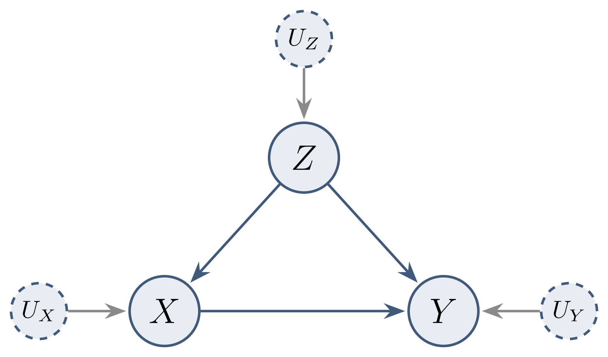
\[ \begin{aligned} Z &:= U_Z \\ X &:= 2Z + U_X \\ Y &:= 3X + Z + U_Y, \qquad U_Z, U_X, U_Y \overset{iid}{\sim} \mathcal N(0, 1) \end{aligned} \]

Causal DAG: from SCM to graph

  • Edge \(V_i \to V_j\) iff \(V_i\) argument of \(f_j\)
  • Markovian SCM → observational law factorises along the DAG
  • Same DAG as a Bayesian network, stronger semantics

Causal model vs graphical model Graphical model: describes one distribution. Causal model: also predicts the distributions after interventions.

Interventions

Conditioning vs intervening

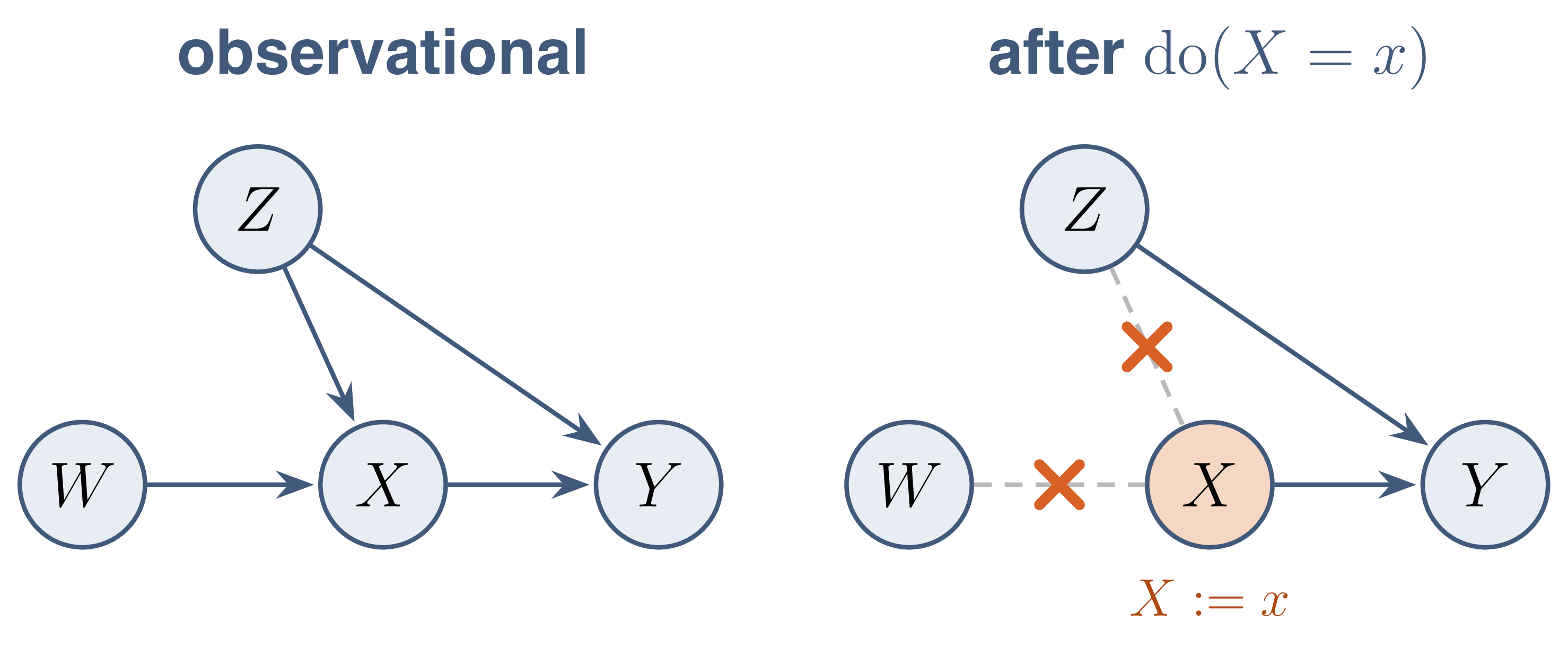
  • Conditioning \(P(Y \mid X = x)\): sub-population with \(X = x\), graph intact
  • Intervening \(P(Y \mid do(X = x))\): \(X\) forced to \(x\) for everyone
  • Confounder \(Z\): association through \(X \leftarrow Z \to Y\) only in the first case

\[ P(Y \mid X = x) \neq P(Y \mid do(X = x)) \quad \text{in general} \]

Modularity

Each mechanism \(f_j\), or conditional \(P(v_j \mid v_{pa(j)})\), is an autonomous module: an intervention on one variable leaves all other modules unchanged.

  • \(do(X = x)\): equation of \(X\) replaced by \(X := x\)
  • Graph surgery: arrows into \(X\) deleted → \(G_{\overline X}\)

Truncated factorisation

Under modularity, the interventional law is the observational factorisation with the factor of the intervened variable removed.

\[ P\big(v \mid do(X = x)\big) = \mathbb 1(x_v = x) \prod_{j \,:\, V_j \neq X} P\big(v_j \mid v_{pa(j)}\big) \]

Causal effect on \(Y\): marginalisation of the truncated product over \(V \setminus \{X, Y\}\).

Confounder: adjustment by \(Z\)

DAG \(Z \to X\), \(Z \to Y\), \(X \to Y\):

\[ \begin{aligned} P(y \mid do(x)) &= \textstyle\sum_z P(z)\, P(y \mid x, z) \\ P(y \mid x) &= \textstyle\sum_z P(z \mid x)\, P(y \mid x, z) \end{aligned} \]

Difference: weights \(P(z)\) vs \(P(z \mid x)\), exactly the mechanism of Simpson’s paradox.

Kidney stones: effect under intervention

\[ \begin{aligned} P(R \mid do(\text{new})) &= 0.51 \times 0.93 + 0.49 \times 0.73 = 0.83 \\ P(R \mid do(\text{standard})) &= 0.51 \times 0.87 + 0.49 \times 0.69 = 0.78 \end{aligned} \]

  • Conditioning, weights \(P(s \mid t)\): \(0.78\) vs \(0.83\), difference \(-0.05\)
  • Intervention, weights \(P(s)\), \(P(\text{small}) = 357/700\): \(0.83\) vs \(0.78\), difference \(+0.05\)

Simpson’s paradox resolved Same stratified rates, other weights: +5 points for the new drug.

Linear example: regression slope vs causal effect

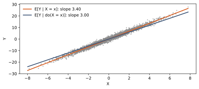
Theory: \(\mathbb E[Y \mid X = x] = 3x + \mathbb E[Z \mid X = x] = 3.4\,x\), \(\;\mathbb E[Y \mid do(X = x)] = 3x\).

Identification by adjustment

Backdoor path

  • Path between \(X\) and \(Y\) starting with an arrow into \(X\): \(X \leftarrow \cdots\; Y\)
  • Carrier of non-causal association
  • Causal paths: directed paths \(X \to \cdots \to Y\)

Backdoor criterion

A set \(Z\) satisfies the backdoor criterion relative to \((X, Y)\) when it contains no descendant of \(X\) and blocks every backdoor path between \(X\) and \(Y\).

\[ \text{(i) } Z \cap de(X) = \emptyset, \qquad \text{(ii) } Z \text{ blocks every path } X \leftarrow \cdots\; Y \]

Backdoor adjustment formula \[ P\big(y \mid do(x)\big) = \sum_z P(y \mid x, z)\, P(z) \]

Backdoor formula: proof sketch

\(W = V \setminus (\{X, Y\} \cup Z)\), truncated factorisation:

\[ P(y \mid do(x)) = \sum_{z, w} P(y \mid x, z, w)\; P(z, w \mid do(x)) \]

      • DAG structure: \(Y \perp W \mid X, Z\) in \(G_{\underline X}\) → \(P(y \mid x, z, w) = P(y \mid x, z)\)
  • (i): \(Z, W\) non-descendants → \(P(z, w \mid do(x)) = P(z, w)\)
  • Sum over \(w\) → formula

Rigorous version: rules 2 and 3 of the do-calculus (Pearl, 1995).

Several confounders

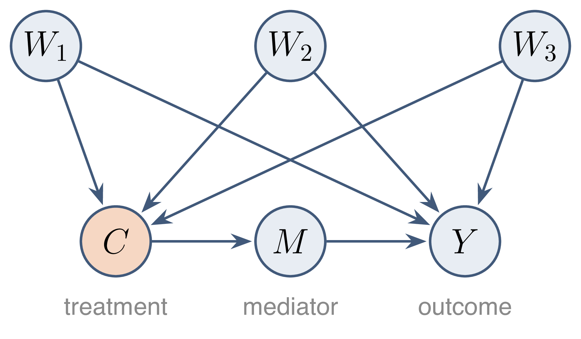
  • Treatment \(C\), outcome \(Y\), mediator \(M\)
  • Backdoor paths \(C \leftarrow W_k \to Y\)
  • Valid set: \(\{W_1, W_2, W_3\}\)
  • \(M\): descendant of \(C\), never adjusted

\[ P(y \mid do(c)) = \sum_{w} P(y \mid c, w)\, P(w) \]

Bad controls

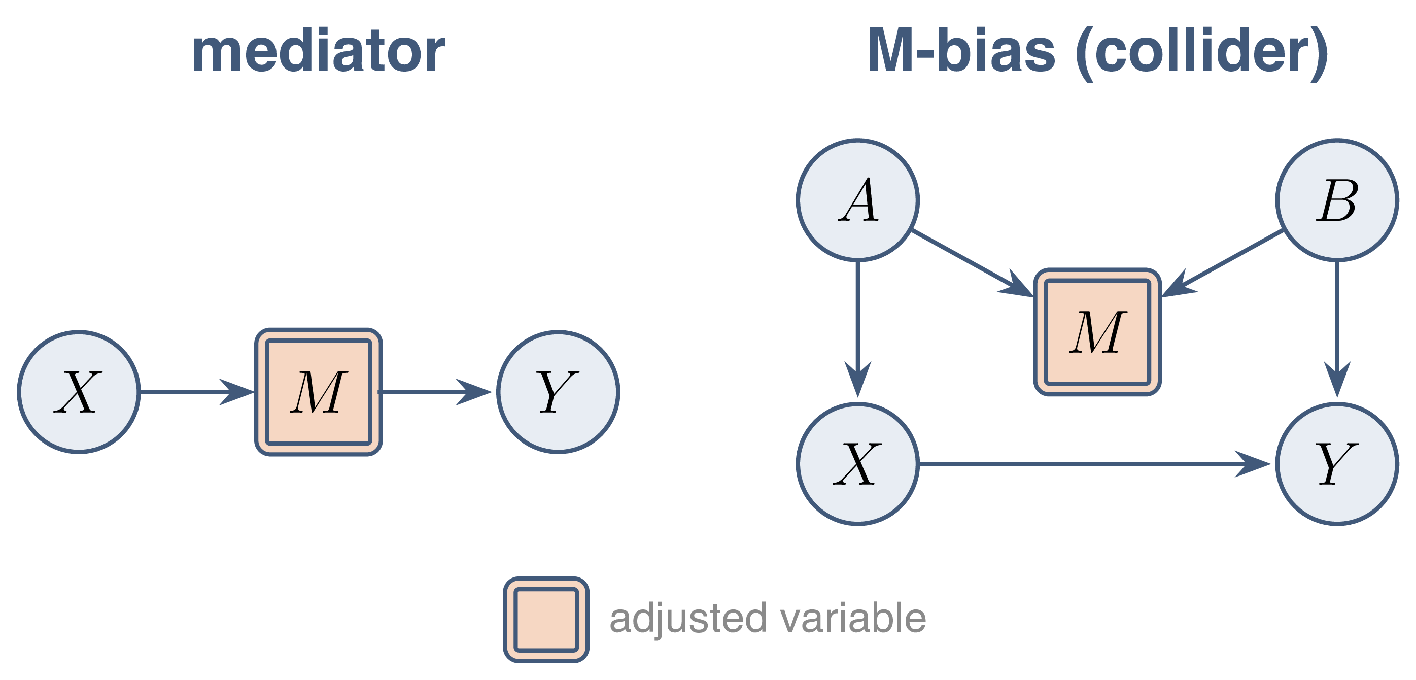
  • Mediator \(M\): part of the effect removed
  • Collider \(M\) (M-bias): adjustment opens \(X \leftarrow A \to M \leftarrow B \to Y\)
  • Rule: adjustment set chosen from the graph, not from correlations

Frontdoor criterion

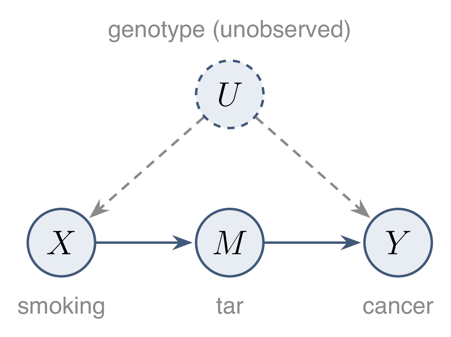
Unobserved confounder \(U\), mediator \(M\) intercepting all causal paths.

  • \(M\) intercepts every directed path \(X \to Y\)
  • No unblocked backdoor path \(X \to M\)
  • Every backdoor path \(M \to Y\) blocked by \(X\)
Frontdoor adjustment formula

Under the frontdoor criterion, the causal effect is identified in two steps: effect of \(X\) on \(M\), then of \(M\) on \(Y\) adjusted on \(X\).

\[ P\big(y \mid do(x)\big) = \sum_m P(m \mid x) \sum_{x'} P(y \mid x', m)\, P(x') \]

  • Step 1: \(P(m \mid do(x)) = P(m \mid x)\), no backdoor path
  • Step 2: \(P(y \mid do(m)) = \sum_{x'} P(y \mid x', m) P(x')\), backdoor via \(X\)

Instrumental variables and Mendelian randomisation

Unobserved confounding

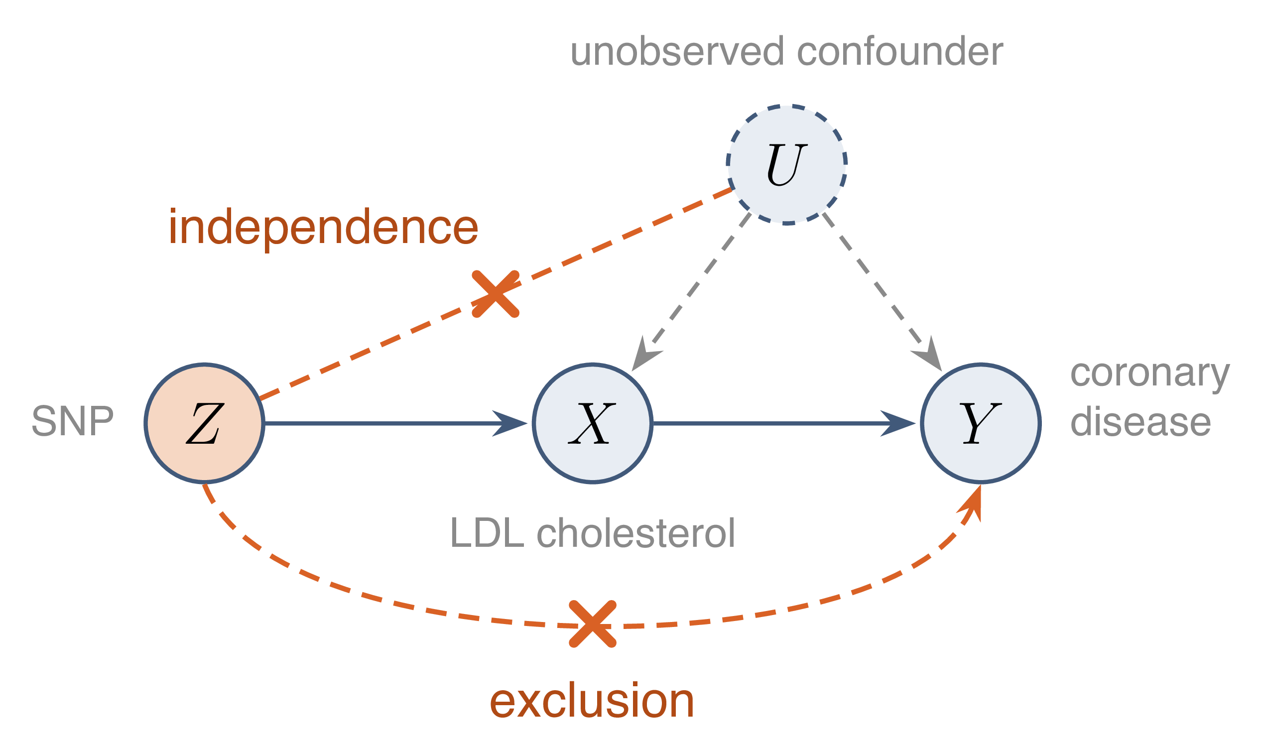
  • Exposure \(X\) (LDL cholesterol), outcome \(Y\) (coronary disease)
  • Confounder \(U\) (lifestyle, socio-economic status): unobserved
  • No backdoor set available → adjustment impossible

Instrumental variable

A variable \(Z\) is an instrument for the effect of \(X\) on \(Y\) when it is associated with \(X\), independent of the confounders, and acts on \(Y\) only through \(X\).

\[ \text{(relevance) } Z \not\perp X, \qquad \text{(independence) } Z \perp U, \qquad \text{(exclusion) } Z \perp_{G_{\overline X}} Y \]

Mendelian randomisation

  • Instrument \(Z\): genetic variant (SNP, 0/1/2 risk alleles)
  • Alleles randomly allocated at meiosis → natural randomised trial
  • Independence: genotype fixed at conception, before \(U\)
  • Threats: pleiotropy (exclusion), population stratification, linkage disequilibrium

Linear model: Wald ratio

\[ X = \beta_{ZX} Z + \gamma_X U + \varepsilon_X, \qquad Y = \alpha X + \gamma_Y U + \varepsilon_Y \]

  • \(\operatorname{Cov}(Z, X) = \beta_{ZX} \operatorname{Var} Z\)
  • \(\operatorname{Cov}(Z, Y) = \alpha\, \beta_{ZX} \operatorname{Var} Z\), since \(Z \perp U\) and exclusion

Wald ratio \[ \alpha = \frac{\operatorname{Cov}(Z, Y)}{\operatorname{Cov}(Z, X)} = \frac{\beta_{ZY}}{\beta_{ZX}} \]

Naive regression vs instrument

import numpy as np
rng = np.random.default_rng(7); N = 20_000
Z = rng.binomial(2, 0.3, N)                    # genotype
U = rng.standard_normal(N)                     # unobserved confounder
X = 0.5 * Z + U + rng.standard_normal(N)       # exposure
Y = 0.2 * X + 1.5 * U + rng.standard_normal(N) # outcome, true effect 0.2
ols = np.cov(X, Y)[0, 1] / np.var(X, ddof=1)
wald = np.cov(Z, Y)[0, 1] / np.cov(Z, X)[0, 1]
print(f"OLS: {ols:.3f}   Wald ratio: {wald:.3f}")
OLS: 0.912   Wald ratio: 0.185
  • OLS: biased by \(U\)
  • Wald ratio: consistent; variance large if weak instrument

Counterfactuals

Counterfactual question

  • Patient treated (\(X = 1\)), recovered (\(Y = 1\))
  • Question: recovery of this patient without treatment?
  • Notation: \(Y_{x}\), value of \(Y\) had \(X\) been set to \(x\)
Population Individual
intervention \(P(Y \mid do(X = x))\) —
counterfactual — \(Y_{x}(u)\) given the facts

Counterfactuals in an SCM

The counterfactual value is obtained by keeping the exogenous noises of the individual and replacing the equation of \(X\).

  1. Abduction: noises \(u\) inferred from the observed facts
  2. Action: equation of \(X\) replaced by \(X := x\)
  3. Prediction: modified equations solved with the same \(u\)

\[ Y_x(u) = f_Y\big(x, Z(u), u_Y\big), \qquad u \text{ fixed by the facts} \]

Counterfactual: worked example

SCM: \(Z := U_Z\), \(X := 2Z + U_X\), \(Y := 3X + Z + U_Y\). Facts for one individual: \(z = 0.5\), \(x = 2\), \(y = 7\).

  1. Abduction: \(u_Z = 0.5\), \(u_X = 2 - 1 = 1\), \(u_Y = 7 - 6 - 0.5 = 0.5\)
  2. Action: \(X := 0\)
  3. Prediction: \(Y_{X=0} = 3 \cdot 0 + 0.5 + 0.5 = 1\)

Interventional mean \(\mathbb E[Y \mid do(X = 0)] = 0\): population answer ≠ individual answer.

Counterfactuals need the full SCM, not only the DAG and \(P\).