Markov random fields and Gaussian graphical models
Lecture 3 — Causality and Graphical Models
M2 Data Science — Université d’Évry
Prior knowledge
Lectures 1 and 2
- DAG factorisation: \(p(x) = \prod_t p(x_t \mid x_{pa(t)})\)
- Gaussian Bayesian network: \(\Sigma = (I - W)^{-1} S^2 (I - W)^{-\top}\)
- Chain, fork: conditioning blocks; collider: conditioning opens
- d-separation \(\Rightarrow\) conditional independence (global Markov property)
- Markov blanket: parents, children, co-parents
- Markov equivalence: same skeleton + same v-structures → CPDAG
Markov random fields
Undirected graphs: motivation
- DAG: arrows imposed, often arbitrary (pixels, spins, co-expressed genes)
- Symmetric interactions → undirected edges
- Independence read by plain graph separation
Graph separation
\(C\) separates \(A\) from \(B\) when every path from \(A\) to \(B\) goes through \(C\).
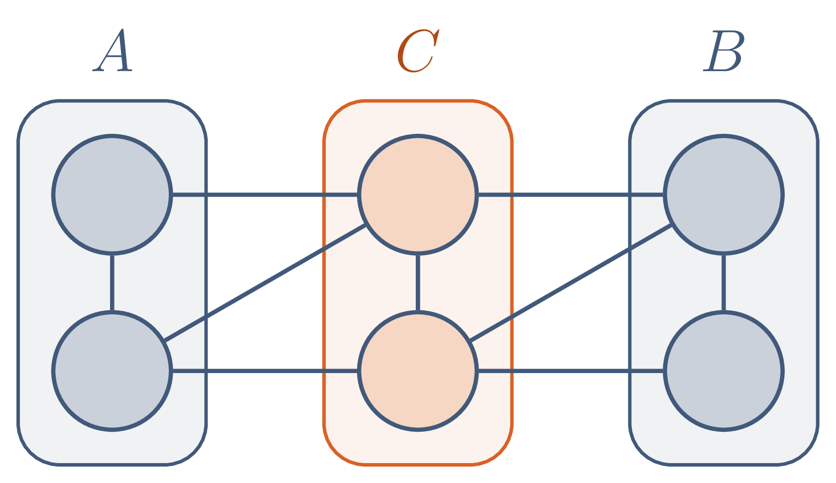
Markov properties of an undirected graph
| Property | Statement |
|---|---|
| global | \(C\) separates \(A\) and \(B\) \(\Rightarrow\) \(X_A \perp X_B \mid X_C\) |
| local | \(X_v \perp X_{V \setminus (\{v\} \cup N(v))} \mid X_{N(v)}\) |
| pairwise | \(u \not\sim v\) \(\Rightarrow\) \(X_u \perp X_v \mid X_{V \setminus \{u, v\}}\) |
- global \(\Rightarrow\) local \(\Rightarrow\) pairwise
- Equivalence for positive densities
- Markov blanket of \(v\): its neighbours \(N(v)\)
Gibbs distribution
A Gibbs distribution for \(G\) is a product of non-negative potentials over the cliques of \(G\), normalised by the partition function.
\[ p(x) = \frac{1}{Z} \prod_{c \in \mathcal C(G)} \psi_c(x_c), \qquad Z = \sum_x \prod_{c \in \mathcal C(G)} \psi_c(x_c) \]
- Potential: compatibility, not a probability
- \(Z\): sum over \(K^V\) configurations → main computational obstacle
Hammersley–Clifford theorem
A strictly positive distribution satisfies the global Markov property of \(G\) if and only if it is a Gibbs distribution for \(G\).
\[ p > 0: \quad p \text{ globally Markov w.r.t. } G \iff p(x) = \frac{1}{Z} \prod_{c \in \mathcal C(G)} \psi_c(x_c) \]
Hammersley–Clifford: idea of the proof
- \(\Leftarrow\): direct, separation splits the product
- \(\Rightarrow\): \(Q(x) = \log p(x)/p(0)\), expansion on all subsets \(A \subseteq V\)
\[ Q(x) = \sum_{A \subseteq V} \textstyle\prod_{i \in A} x_i\; G_A(x_A) \]
- \(l \notin N(i)\): \(\dfrac{p(x)}{p(x^{i})} = \dfrac{p(x_i \mid x_{N(i)})}{p(0 \mid x_{N(i)})}\) free of \(x_l\)
- → \(G_A = 0\) unless \(A\) is a clique
Moralisation
Moral graph of a DAG: parents of each node married, then orientations dropped.
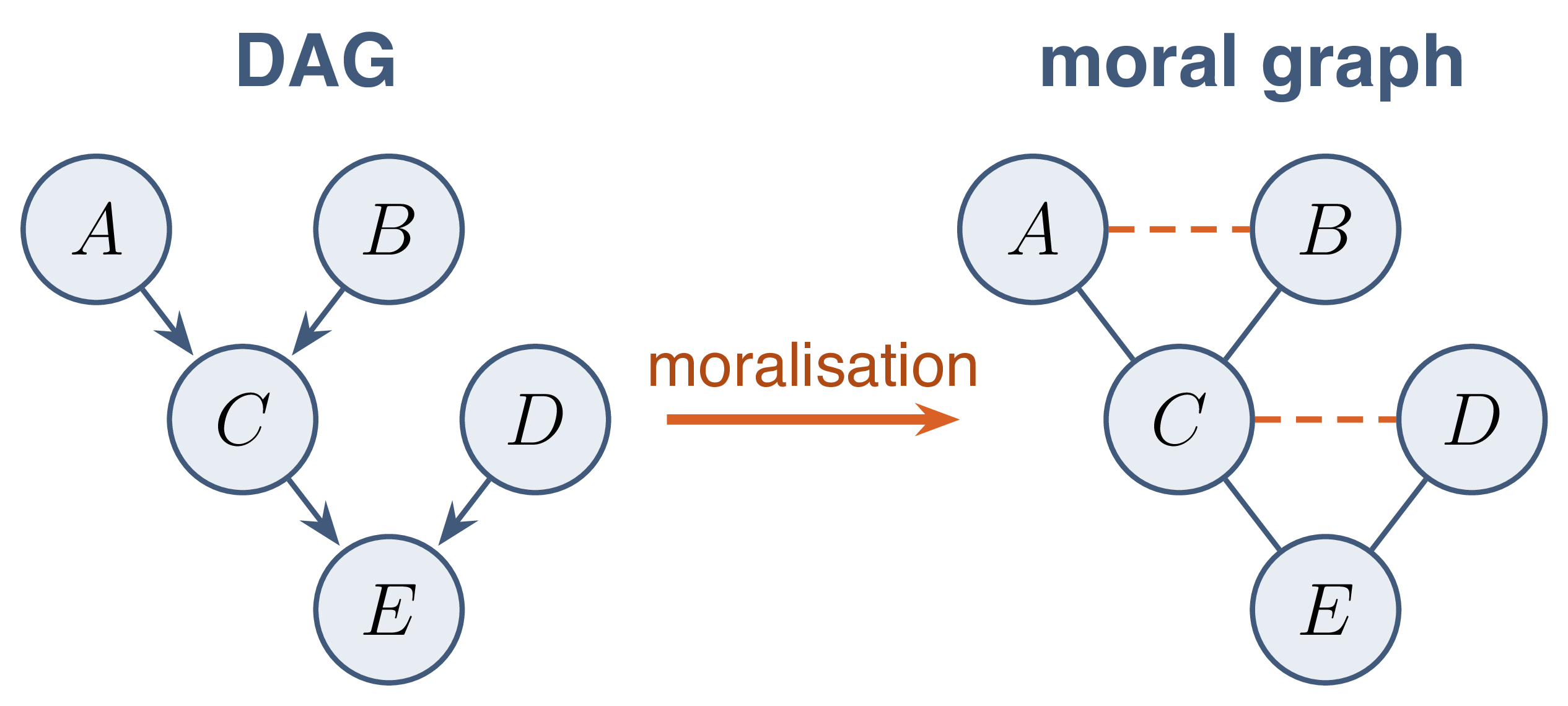
Proposition A distribution factorising according to a DAG \(G\) is a Gibbs distribution for its moral graph \(G^m\).
Price: lost independences (v-structures).
Ising model
- Spins \(x_s \in \{-1, +1\}\) on a grid
- Pairwise potentials \(\psi_{st}(x_s, x_t) = e^{w_{st} x_s x_t}\), external field \(b\)
\[ p(x) = \frac{1}{Z} \exp\Big(\sum_{s \sim t} w_{st}\, x_s x_t + \sum_s b_s x_s\Big) \]
- \(w_{st} = \beta > 0\): aligned neighbours (ferromagnet)
- \(Z\): sum over \(2^V\) configurations, intractable
Ising: conditional distribution of one site
With \(w_{st} = \beta\) and \(b_s = \alpha\), a site depends on the rest only through the sum of its neighbours.
\[ p(x_i = 1 \mid x_{-i}) = \frac{e^{\alpha + \beta m_i}}{e^{\alpha + \beta m_i} + e^{-\alpha - \beta m_i}} = \sigma\big(2(\alpha + \beta m_i)\big), \qquad m_i = \sum_{j \sim i} x_j \]
\(Z\) cancels: local computation only.
Gibbs sampler
- Initial configuration \(x^{(0)}\)
- Sweep over sites, each site drawn from \(p(x_i \mid x_{N(i)})\)
- Repeat → Markov chain with stationary law \(p\)
- Checkerboard updates: half of the sites in parallel
- Burn-in, autocorrelation: usual MCMC caveats
Ising samples
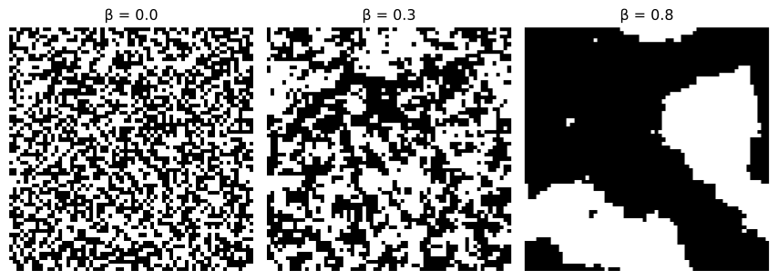
Critical value (2D grid, infinite size): \(\beta_c = \tfrac12 \log(1 + \sqrt 2) \approx 0.44\).
Gaussian graphical models
Multivariate Gaussian and precision matrix
\[ f(x) = \frac{1}{(2\pi)^{p/2} |\Sigma|^{1/2}} \exp\Big(-\tfrac12 (x - \mu)^\top K (x - \mu)\Big), \qquad K = \Sigma^{-1} \]
- \(K\): precision (concentration) matrix
- Exponent: only pairwise terms \(x_j K_{jk} x_k\) → Gibbs distribution with cliques of size \(\leq 2\)
Conditional Gaussian
For a Gaussian vector split into blocks \(A\) and \(B\), the law of \(X_A\) given \(X_B = b\) is Gaussian.
\[ \begin{aligned} X_A \mid X_B = b \;&\sim\; \mathcal N\big(\mu_A + \Sigma_{AB} \Sigma_{BB}^{-1} (b - \mu_B),\ \Sigma_{A \mid B}\big) \\ \Sigma_{A \mid B} &= \Sigma_{AA} - \Sigma_{AB} \Sigma_{BB}^{-1} \Sigma_{BA} = (K_{AA})^{-1} \end{aligned} \]
Last equality: Schur complement.
Zeros of the precision matrix
In a Gaussian vector, two variables are independent given all the others if and only if the corresponding entry of \(K\) is zero.
\[ K_{ij} = 0 \iff X_i \perp X_j \mid X_{V \setminus \{i, j\}} \]
Partial correlation: \(\rho_{ij \cdot V \setminus\{i,j\}} = -K_{ij} / \sqrt{K_{ii} K_{jj}}\).
Gaussian graphical model Graph \(G\) with edge \(i - j\) iff \(K_{ij} \neq 0\): support of the precision matrix.
Covariance vs precision
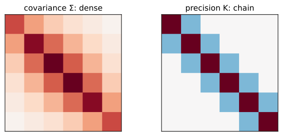
Marginal correlation everywhere, conditional dependence only along the chain.
From a Gaussian DAG to its moral graph
Gaussian Bayesian network \(x - \mu = W(x - \mu) + S z\):
\[ K = (I - W)^\top S^{-2} (I - W) \]
- \(K_{ij} \neq 0\) (generic weights) iff \(i, j\) adjacent or co-parents
- Support of \(K\) = moral graph of the DAG
- GGM: undirected shadow of the causal structure
Covariance selection: known graph
Sample \(x_1, \dots, x_N\), empirical covariance \(S\). Log-likelihood up to constants:
\[ \ell(K) = \frac N2 \big(\log\det K - \operatorname{tr}(S K)\big), \qquad \nabla_K \ell \propto K^{-1} - S \]
Maximum likelihood under the constraint \(K_{st} = 0\) for \(s \not\sim t\):
- \(\hat\Sigma_{st} = S_{st}\) on edges and diagonal
- \(\hat K_{st} = 0\) off edges
- \(\hat\Sigma\): positive definite completion of \(S\) (Dempster, 1972)
Graphical lasso: unknown graph
The graphical lasso penalises the \(\ell_1\) norm of the precision matrix to obtain a sparse estimate.
\[ \hat K_\lambda = \arg\min_{K \succ 0}\; -\log\det K + \operatorname{tr}(S K) + \lambda \sum_{s \neq t} |K_{st}| \]
- \(\lambda\) large → sparse graph
- Defined even for \(p > N\)
- Friedman, Hastie & Tibshirani (2008): block coordinate descent
Graphical lasso algorithm
Subgradient condition: \(W - S - \lambda\, \Gamma = 0\), \(W = K^{-1}\), \(\Gamma_{st} \in \partial|K_{st}|\).
- \(W \leftarrow S + \lambda I\) (diagonal fixed)
- For each column \(j\): lasso \(\min_\beta \tfrac12 \beta^\top W_{11} \beta - \beta^\top s_{12} + \lambda \|\beta\|_1\)
- Update \(w_{12} = W_{11} \hat\beta\); loop until convergence
- Recovery: \(\hat k_{22} = 1/(w_{22} - w_{12}^\top \hat\beta)\), \(\hat k_{12} = -\hat\beta\, \hat k_{22}\)
Graphical lasso on simulated data
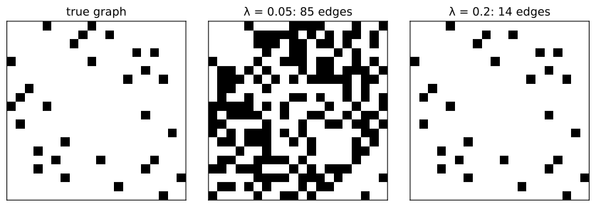
Choice of \(\lambda\): cross-validation, StARS, BIC.
Graph learned: conditional dependences, not causal directions.
Appendix: Boltzmann machines
Boltzmann machine
Binary units \(x \in \{0, 1\}^p\), symmetric weights \(w_{jk}\), \(w_{jj} = 0\):
\[ p(x) = \frac{1}{Z} \exp\Big(\sum_j \alpha_j x_j + \sum_{j < k} w_{jk}\, x_j x_k\Big) \]
- Each conditional: logistic regression on the other units
- Log-likelihood gradient: \(\mathbb E_{\text{data}}[x_j x_k] - \mathbb E_{\text{model}}[x_j x_k]\)
- Model expectation: Gibbs sampling, costly
Restricted Boltzmann machine
- Visible units \(v\), hidden units \(h\), edges only between layers
- \(v \perp\) given \(h\), \(h \perp\) given \(v\) → block Gibbs sampling
\[ p(h_j = 1 \mid v) = \sigma\big(c_j + \textstyle\sum_i w_{ij} v_i\big), \qquad p(v_i = 1 \mid h) = \sigma\big(b_i + \textstyle\sum_j w_{ij} h_j\big) \]
- Contrastive divergence (CD-\(k\)): \(k\) Gibbs steps from the data
- Historical building block of deep belief networks (Hinton, 2006)