Interventions, Mendelian randomisation and causal discovery

M2 GENIOMHE — Session 3

Christophe Ambroise

M2 GENIOMHE — Université d’Évry

Prior knowledge

Sessions 1 and 2

  • d-separation; Markov equivalence → CPDAG
  • Gaussian graphical model: \(K_{ij} = 0 \iff X_i \perp X_j \mid X_{\text{rest}}\)
  • Graphical lasso: sparse precision matrix
  • PC algorithm: skeleton, v-structures, Meek rules → CPDAG
  • Gaussian linear SEM: direction of \(X_1 - X_2\) not identifiable

Structural causal models

Structural causal model

A structural causal model (SCM) generates each endogenous variable by a deterministic mechanism of its direct causes and of an exogenous noise.

\[ \mathcal M = (U, V, F, P_U): \qquad V_j := f_j\big(V_{pa(j)},\, U_j\big), \quad j = 1, \dots, p \]

  • \(V\): endogenous variables, modelled
  • \(U\): exogenous variables, causes left outside the model
  • \(U_j\) jointly independent → Markovian SCM

SCM example

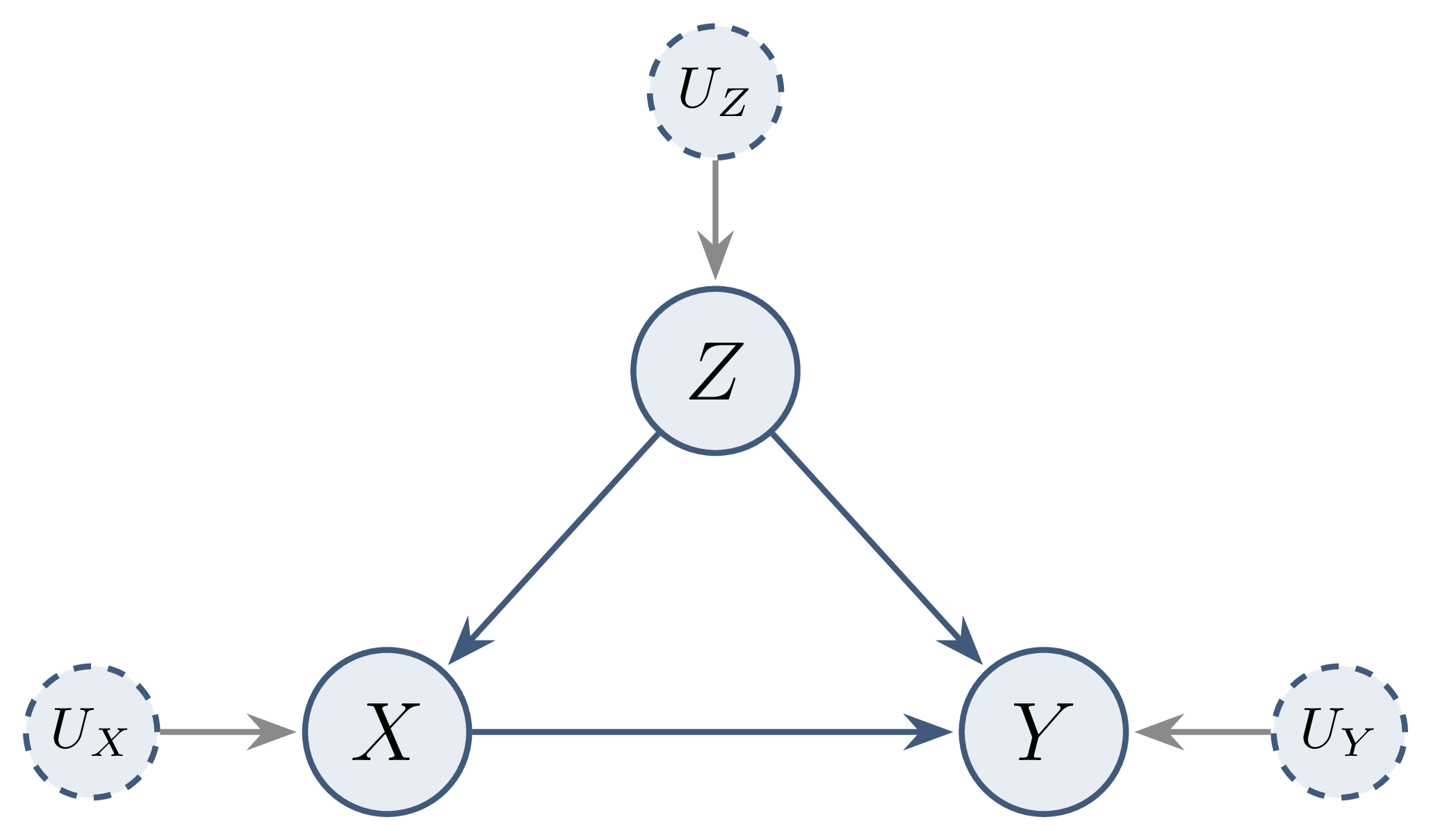
\[ \begin{aligned} Z &:= U_Z \\ X &:= 2Z + U_X \\ Y &:= 3X + Z + U_Y, \qquad U_Z, U_X, U_Y \overset{iid}{\sim} \mathcal N(0, 1) \end{aligned} \]

Causal DAG: from SCM to graph

  • Edge \(V_i \to V_j\) iff \(V_i\) argument of \(f_j\)
  • Markovian SCM → observational law factorises along the DAG
  • Same DAG as a Bayesian network, stronger semantics

Causal model vs graphical model Graphical model: describes one distribution. Causal model: also predicts the distributions after interventions.

Interventions

Conditioning vs intervening

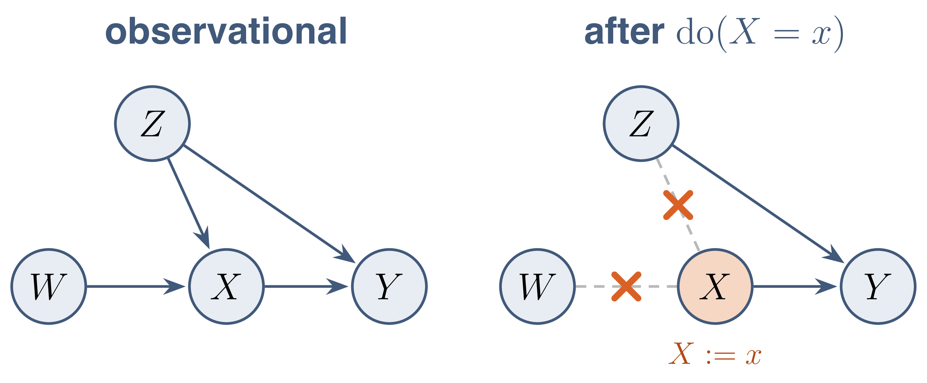
  • Conditioning \(P(Y \mid X = x)\): sub-population with \(X = x\), graph intact
  • Intervening \(P(Y \mid do(X = x))\): \(X\) forced to \(x\) for everyone
  • Confounder \(Z\): association through \(X \leftarrow Z \to Y\) only in the first case

\[ P(Y \mid X = x) \neq P(Y \mid do(X = x)) \quad \text{in general} \]

Modularity

Each mechanism \(f_j\), or conditional \(P(v_j \mid v_{pa(j)})\), is an autonomous module: an intervention on one variable leaves all other modules unchanged.

  • \(do(X = x)\): equation of \(X\) replaced by \(X := x\)
  • Graph surgery: arrows into \(X\) deleted → \(G_{\overline X}\)

Truncated factorisation

Under modularity, the interventional law is the observational factorisation with the factor of the intervened variable removed.

\[ P\big(v \mid do(X = x)\big) = \mathbb 1(x_v = x) \prod_{j \,:\, V_j \neq X} P\big(v_j \mid v_{pa(j)}\big) \]

Causal effect on \(Y\): marginalisation of the truncated product over \(V \setminus \{X, Y\}\).

Confounder: adjustment by \(Z\)

DAG \(Z \to X\), \(Z \to Y\), \(X \to Y\):

\[ \begin{aligned} P(y \mid do(x)) &= \textstyle\sum_z P(z)\, P(y \mid x, z) \\ P(y \mid x) &= \textstyle\sum_z P(z \mid x)\, P(y \mid x, z) \end{aligned} \]

Difference: weights \(P(z)\) vs \(P(z \mid x)\), exactly the mechanism of Simpson’s paradox.

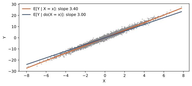
Linear example: regression slope vs causal effect

Theory: \(\mathbb E[Y \mid X = x] = 3x + \mathbb E[Z \mid X = x] = 3.4\,x\), \(\;\mathbb E[Y \mid do(X = x)] = 3x\).

Identification by adjustment

Backdoor path

  • Path between \(X\) and \(Y\) starting with an arrow into \(X\): \(X \leftarrow \cdots\; Y\)
  • Carrier of non-causal association
  • Causal paths: directed paths \(X \to \cdots \to Y\)

Backdoor criterion

A set \(Z\) satisfies the backdoor criterion relative to \((X, Y)\) when it contains no descendant of \(X\) and blocks every backdoor path between \(X\) and \(Y\).

\[ \text{(i) } Z \cap de(X) = \emptyset, \qquad \text{(ii) } Z \text{ blocks every path } X \leftarrow \cdots\; Y \]

Backdoor adjustment formula \[ P\big(y \mid do(x)\big) = \sum_z P(y \mid x, z)\, P(z) \]

Several confounders

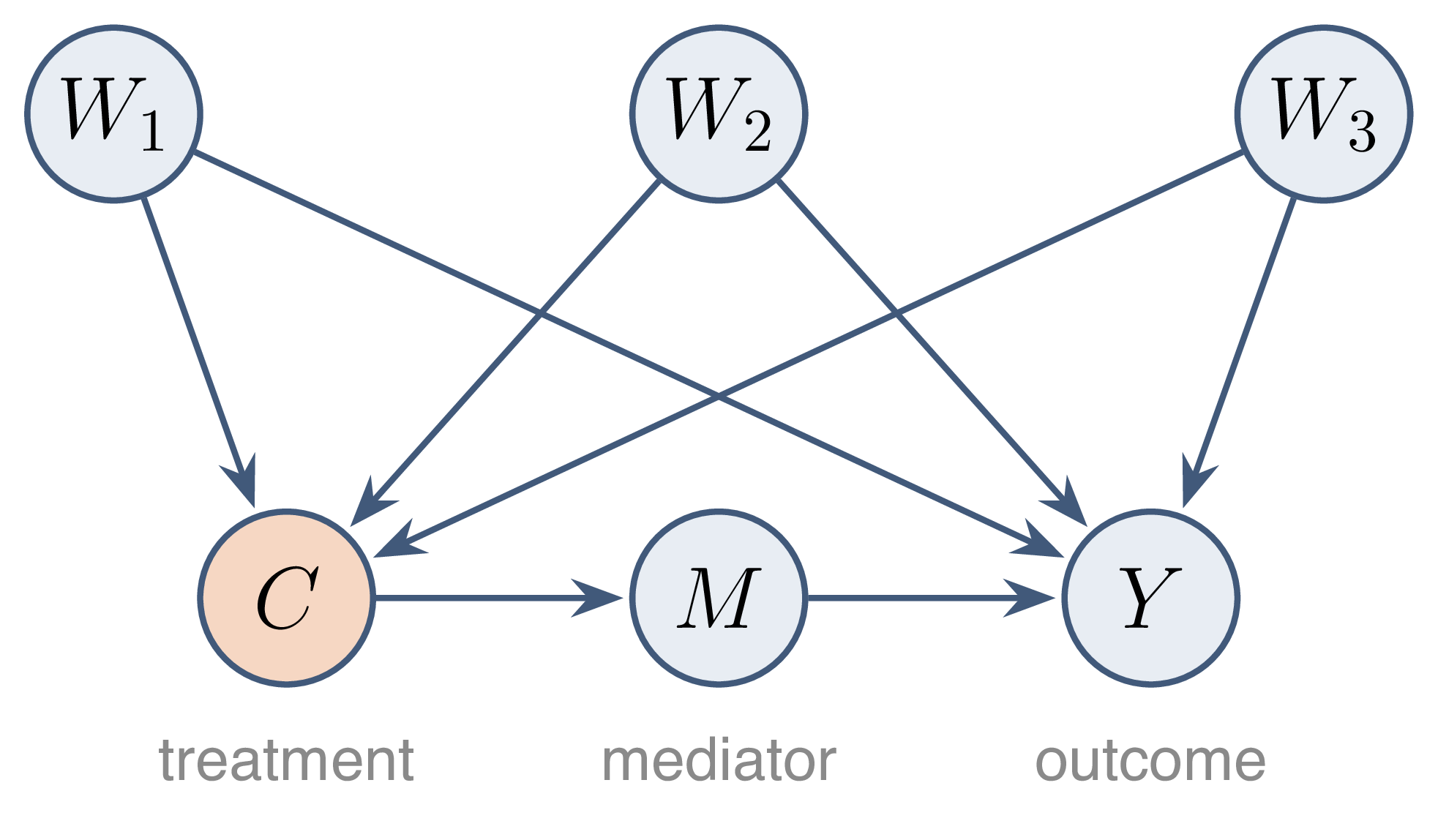
  • Treatment \(C\), outcome \(Y\), mediator \(M\)
  • Backdoor paths \(C \leftarrow W_k \to Y\)
  • Valid set: \(\{W_1, W_2, W_3\}\)
  • \(M\): descendant of \(C\), never adjusted

\[ P(y \mid do(c)) = \sum_{w} P(y \mid c, w)\, P(w) \]

Bad controls

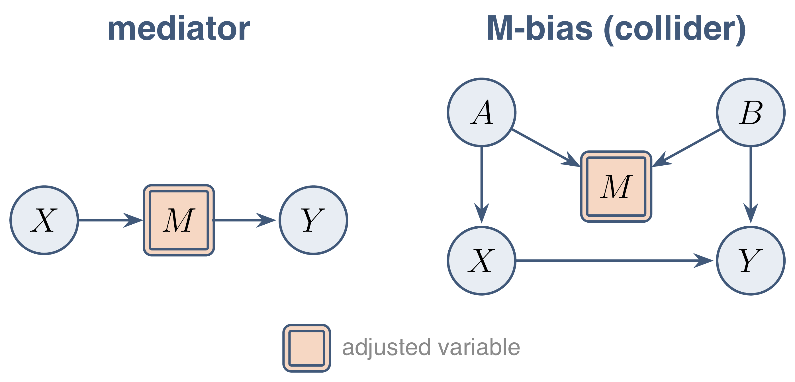
  • Mediator \(M\): part of the effect removed
  • Collider \(M\) (M-bias): adjustment opens \(X \leftarrow A \to M \leftarrow B \to Y\)
  • Rule: adjustment set chosen from the graph, not from correlations

Instrumental variables and Mendelian randomisation

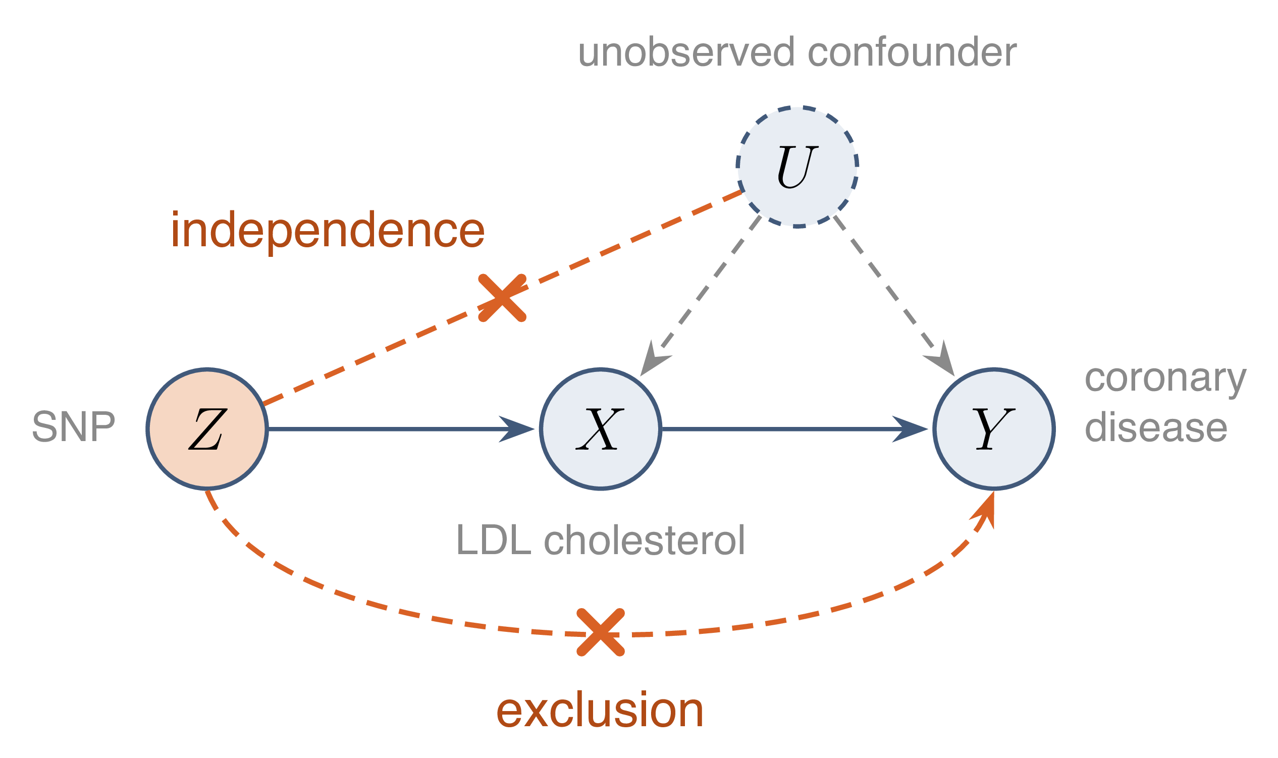
Unobserved confounding

  • Exposure \(X\) (LDL cholesterol), outcome \(Y\) (coronary disease)
  • Confounder \(U\) (lifestyle, socio-economic status): unobserved
  • No backdoor set available → adjustment impossible

Instrumental variable

A variable \(Z\) is an instrument for the effect of \(X\) on \(Y\) when it is associated with \(X\), independent of the confounders, and acts on \(Y\) only through \(X\).

\[ \text{(relevance) } Z \not\perp X, \qquad \text{(independence) } Z \perp U, \qquad \text{(exclusion) } Z \perp_{G_{\overline X}} Y \]

Mendelian randomisation

  • Instrument \(Z\): genetic variant (SNP, 0/1/2 risk alleles)
  • Alleles randomly allocated at meiosis → natural randomised trial
  • Independence: genotype fixed at conception, before \(U\)
  • Threats: pleiotropy (exclusion), population stratification, linkage disequilibrium

Linear model: Wald ratio

\[ X = \beta_{ZX} Z + \gamma_X U + \varepsilon_X, \qquad Y = \alpha X + \gamma_Y U + \varepsilon_Y \]

  • \(\operatorname{Cov}(Z, X) = \beta_{ZX} \operatorname{Var} Z\)
  • \(\operatorname{Cov}(Z, Y) = \alpha\, \beta_{ZX} \operatorname{Var} Z\), since \(Z \perp U\) and exclusion

Wald ratio \[ \alpha = \frac{\operatorname{Cov}(Z, Y)}{\operatorname{Cov}(Z, X)} = \frac{\beta_{ZY}}{\beta_{ZX}} \]

Naive regression vs instrument

import numpy as np
rng = np.random.default_rng(7); N = 20_000
Z = rng.binomial(2, 0.3, N)                    # genotype
U = rng.standard_normal(N)                     # unobserved confounder
X = 0.5 * Z + U + rng.standard_normal(N)       # exposure
Y = 0.2 * X + 1.5 * U + rng.standard_normal(N) # outcome, true effect 0.2
ols = np.cov(X, Y)[0, 1] / np.var(X, ddof=1)
wald = np.cov(Z, Y)[0, 1] / np.cov(Z, X)[0, 1]
print(f"OLS: {ols:.3f}   Wald ratio: {wald:.3f}")
OLS: 0.912   Wald ratio: 0.185
  • OLS: biased by \(U\)
  • Wald ratio: consistent; variance large if weak instrument

Beyond Markov equivalence: LiNGAM

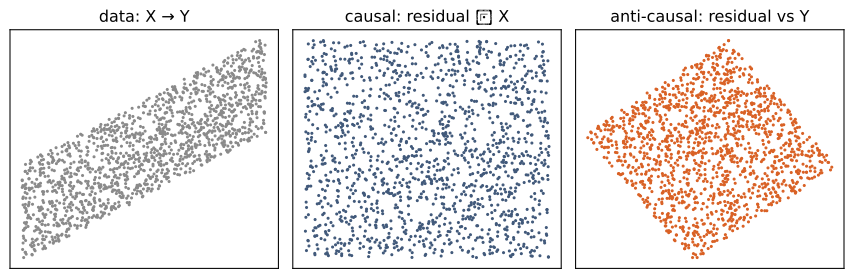
Two variables, one direction?

  • Both residuals uncorrelated with the regressor
  • Only the causal one independent: non-Gaussianity breaks the symmetry

Linear non-Gaussian acyclic model

In LiNGAM, the data follow a linear SEM on a DAG, with mutually independent noises of which at most one is Gaussian.

\[ X = B X + \varepsilon, \qquad B \text{ acyclic (strictly lower triangular up to permutation)}, \qquad \varepsilon_1, \dots, \varepsilon_d \text{ independent} \]

Identifiability (Shimizu et al., 2006) Under these assumptions, \(B\) and the causal order are identifiable from the distribution of \(X\) alone.

DirectLiNGAM

\(X_j\) is exogenous (a source) if and only if every other variable, regressed on \(X_j\), leaves a residual independent of \(X_j\).

\[ X_j \text{ source} \iff \forall\, i \neq j : \quad X_i - \frac{\operatorname{Cov}(X_i, X_j)}{\operatorname{Var} X_j} X_j \;\perp\; X_j \]

  1. Most independent candidate → next variable of the order
  2. Its effect regressed out of all remaining variables
  3. Repeat; then \(B\) by adaptive lasso along the order

Shimizu et al. (2011), JMLR. Python package lingam.

DirectLiNGAM in practice

import numpy as np, lingam
rng = np.random.default_rng(1); n = 2000
e = rng.laplace(size=(n, 4))                     # non-Gaussian noises
x0 = e[:, 0]
x2 = 0.8 * x0 + e[:, 2]
x1 = -0.7 * x2 + e[:, 1]
x3 = 0.5 * x0 + 0.6 * x1 + e[:, 3]
X = np.c_[x0, x1, x2, x3]
model = lingam.DirectLiNGAM().fit(X)
print("order:", [int(i) for i in model.causal_order_])
print(np.round(model.adjacency_matrix_, 2))      # B[j, k] : effect k -> j
order: [0, 2, 1, 3]
[[ 0.    0.    0.    0.  ]
 [ 0.    0.   -0.69  0.  ]
 [ 0.79  0.    0.    0.  ]
 [ 0.51  0.6   0.    0.  ]]

OT-LiNGAM: non-Gaussianity by optimal transport

Measuring non-Gaussianity

  • Classical contrasts: kurtosis, negentropy approximations, likelihood surrogates
  • Choice of a nonlinearity or moment order → method tuned to source shape
  • Wanted: one criterion, no tuning, only finite second moments

Laplante, Ambroise & Humbert, Contrast-free ICA and causal inference via Wasserstein distances to the Gaussian, preprint. Package otlingam.

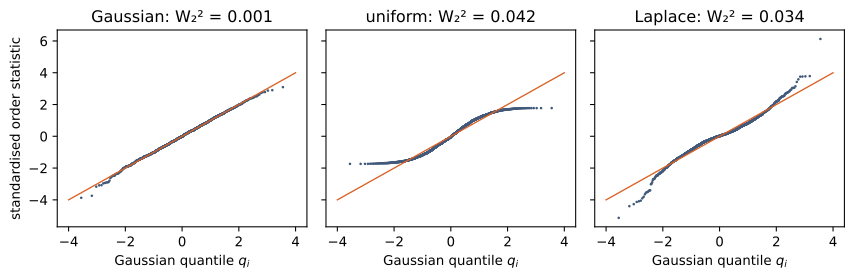
2-Wasserstein distance

The squared 2-Wasserstein distance is the smallest mean squared displacement among all couplings of the two distributions.

\[ \mathcal W_2(\mu, \nu)^2 = \inf_{X \sim \mu,\ Y \sim \nu} \mathbb E\big[(X - Y)^2\big] \overset{\text{dim } 1}{=} \int_0^1 \big(F_\mu^{-1}(u) - F_\nu^{-1}(u)\big)^2\, du \]

  • Dimension 1: optimal coupling = matching of quantiles
  • Non-Gaussianity of \(X\): \(\;\mathcal W_2\big(\operatorname{std}(X), \mathcal N(0, 1)\big)^2\), zero iff \(X\) Gaussian

Non-Gaussianity of three distributions

Mixtures are closer to the Gaussian

Under independence and standardisation, any non-trivial normalised mixture of sources is strictly closer to the Gaussian than the corresponding weighted average of the sources’ distances.

\[ \|\alpha\|_2 = 1,\ \#\{j : \alpha_j \neq 0\} > 1 \;\Longrightarrow\; \mathcal W_2\Big(\sum_j \alpha_j S_j, \mathcal N(0, 1)\Big)^2 < \sum_j \alpha_j^2\, \mathcal W_2\big(S_j, \mathcal N(0, 1)\big)^2 \]

Assumptions: \(S_j\) independent, centred, unit variance, at most one Gaussian.

Wasserstein order objective

For a candidate order \(\sigma\), regress each variable on its predecessors and score the non-Gaussianity of the standardised residuals.

\[ G(\sigma) = \sum_{j=1}^{d} \mathcal W_2\Big(\operatorname{std}\big(R_j(\sigma)\big), \mathcal N(0, 1)\Big)^2, \qquad R_j(\sigma) = X_j - \operatorname{proj}_{\operatorname{span}\{X_k : k \text{ before } j\}} X_j \]

  • Causal order: residuals = structural noises \(\varepsilon_j\)
  • Wrong order: some residual mixes several noises → closer to Gaussian

Identification of causal orders

Theorem (Laplante, Ambroise & Humbert) Under independent, non-degenerate noises with at most one Gaussian, the maximisers of \(G\) are exactly the causal orders of the model.

\[ \arg\max_{\sigma \in \mathfrak S_d} G(\sigma) = \mathcal I^\star = \big\{\sigma : \Pi^\sigma B (\Pi^\sigma)^\top \text{ strictly lower triangular}\big\} \]

Key steps: \(\operatorname{std}(R(\sigma)) = Q^\sigma \operatorname{std}(\varepsilon)\) with \(Q^\sigma\) orthogonal; strict subadditivity; \(Q^\sigma\) signed permutation \(\Rightarrow\) \(\sigma\) causal.

Greedy solver and full pipeline

Greedy OT-LiNGAM: most non-Gaussian standardised residual → next source; its effect regressed out; repeat. Cost \(O(d^2 n \log n)\).

Solver Cost Global optimum
Exhaustive OT-LiNGAM \(O\big(d 2^d (n d^2 + n \log n)\big)\) yes
Greedy OT-LiNGAM \(O(d^2 n \log n)\) no
OT-ICA-LiNGAM \(O(n d^2 + d n \log n)\) / iteration no

Order known → \(B\) by adaptive lasso along the order.

Evaluation: disorder of an order

Number of true edges reversed by the estimated order:

\[ \operatorname{dis}(\hat\sigma) = \#\big\{(k, j) : B_{jk} \neq 0,\ \hat\sigma^{-1}(k) > \hat\sigma^{-1}(j)\big\} \]

  • \(\operatorname{dis}(\hat\sigma) = 0 \iff \hat\sigma\) causal order
  • Simulations of the paper (ER and scale-free graphs, Laplace or Student noises): exhaustive OT-LiNGAM close to zero disorder, robust when some noises approach Gaussianity
  • Continuous methods (DAGMA): degraded under heteroscedastic noises

OT-LiNGAM in practice

import numpy as np
from otlingam import ExhaustiveOTLiNGAM, GreedyOTLiNGAM
from otlingam.utils import disorder
rng = np.random.default_rng(1); n = 2000
e = rng.laplace(size=(n, 4))
x0 = e[:, 0]; x2 = 0.8 * x0 + e[:, 2]
x1 = -0.7 * x2 + e[:, 1]; x3 = 0.5 * x0 + 0.6 * x1 + e[:, 3]
X = np.c_[x0, x1, x2, x3]
B_true = np.zeros((4, 4)); B_true[2, 0], B_true[1, 2], B_true[3, 0], B_true[3, 1] = .8, -.7, .5, .6
for M in (ExhaustiveOTLiNGAM(), GreedyOTLiNGAM()):
    M.fit(X)
    print(type(M).__name__, [int(i) for i in M.causal_order_], "disorder:", disorder(B_true, M.causal_order_))
ExhaustiveOTLiNGAM [0, 2, 1, 3] disorder: 0
GreedyOTLiNGAM [0, 2, 1, 3] disorder: 0

Case study: chloroplast RNA maturation

Biological context

  • Chloroplast transcripts of Arabidopsis thaliana: genes ndhB, ndhD
  • Post-transcriptional maturation: C-to-U editing at specific sites, intron splicing
  • Nanopore long reads: one read = one full-length RNA molecule
  • Each read: snapshot of one molecule at some stage of its maturation

Data: Guilcher et al. (2021), Int. J. Mol. Sci. 22, 11297.

Data: one binary vector per read

  ed1   ed2   ed3   ed4  ed5
False False False  True    ·
 True False     ·     ·    ·
False False False False    ·
False  True False  True    ·
 True False False  True True
False  True  True  True    ·
Gene Reads Events Complete reads
ndhB 1 899 12 editing sites + intron splicing 117
ndhD 7 574 5 editing sites 930

True: event observed; False: not observed; Err: sequencing error; empty: not covered.

Question: chronology of maturation events

  • Order in which sites are edited and the intron spliced
  • Chronology as a causal order of the event variables
  • Snapshot data only: no time stamps

Open problem Can a causal order learned from snapshots of molecules reveal the maturation chronology?

Methodological difficulties

  • Binary variables: linear non-Gaussian model only an approximation
  • Missing blocks: reads truncated, contiguous sites unobserved
  • Errors (Err): measurement noise on some sites
  • Rare events (sites edited in < 10 % of reads)
  • Validation: no ground-truth chronology