Biological networks: Gaussian graphical models and the PC algorithm

M2 GENIOMHE — Session 2

Christophe Ambroise

M2 GENIOMHE — Université d’Évry

Prior knowledge

Session 1

• DAG factorisation: \(p(x) = \prod_t p(x_t \mid x_{pa(t)})\)
• Chain, fork: conditioning blocks; collider: conditioning opens
• d-separation \(\Rightarrow\) conditional independence
• Markov blanket: parents, children, co-parents
• Markov equivalence: same skeleton + same v-structures → CPDAG

Markov random fields

Undirected graphs: motivation

• DAG: arrows imposed, often arbitrary (pixels, spins, co-expressed genes)
• Symmetric interactions → undirected edges
• Independence read by plain graph separation

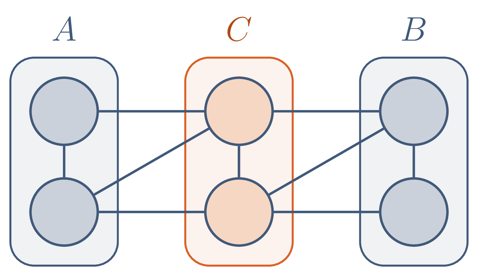
Graph separation

\(C\) separates \(A\) from \(B\) when every path from \(A\) to \(B\) goes through \(C\).

Markov properties of an undirected graph

Property	Statement
global	\(C\) separates \(A\) and \(B\) \(\Rightarrow\) \(X_A \perp X_B \mid X_C\)
local	\(X_v \perp X_{V \setminus (\{v\} \cup N(v))} \mid X_{N(v)}\)
pairwise	\(u \not\sim v\) \(\Rightarrow\) \(X_u \perp X_v \mid X_{V \setminus \{u, v\}}\)

• global \(\Rightarrow\) local \(\Rightarrow\) pairwise
• Equivalence for positive densities
• Markov blanket of \(v\): its neighbours \(N(v)\)

Gibbs distribution

A Gibbs distribution for \(G\) is a product of non-negative potentials over the cliques of \(G\), normalised by the partition function.

\[ p(x) = \frac{1}{Z} \prod_{c \in \mathcal C(G)} \psi_c(x_c), \qquad Z = \sum_x \prod_{c \in \mathcal C(G)} \psi_c(x_c) \]

• Potential: compatibility, not a probability
• \(Z\): sum over \(K^V\) configurations → main computational obstacle

Hammersley–Clifford theorem

A strictly positive distribution satisfies the global Markov property of \(G\) if and only if it is a Gibbs distribution for \(G\).

\[ p > 0: \quad p \text{ globally Markov w.r.t. } G \iff p(x) = \frac{1}{Z} \prod_{c \in \mathcal C(G)} \psi_c(x_c) \]

Moralisation

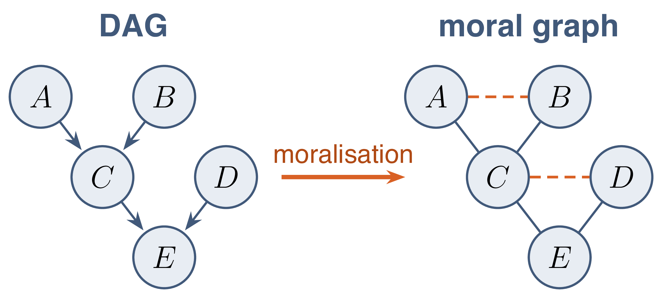
Moral graph of a DAG: parents of each node married, then orientations dropped.

Proposition A distribution factorising according to a DAG \(G\) is a Gibbs distribution for its moral graph \(G^m\).

Price: lost independences (v-structures).

Gaussian graphical models

Multivariate Gaussian and precision matrix

\[ f(x) = \frac{1}{(2\pi)^{p/2} |\Sigma|^{1/2}} \exp\Big(-\tfrac12 (x - \mu)^\top K (x - \mu)\Big), \qquad K = \Sigma^{-1} \]

• \(K\): precision (concentration) matrix
• Exponent: only pairwise terms \(x_j K_{jk} x_k\) → Gibbs distribution with cliques of size \(\leq 2\)

Conditional Gaussian

For a Gaussian vector split into blocks \(A\) and \(B\), the law of \(X_A\) given \(X_B = b\) is Gaussian.

\[ \begin{aligned} X_A \mid X_B = b \;&\sim\; \mathcal N\big(\mu_A + \Sigma_{AB} \Sigma_{BB}^{-1} (b - \mu_B),\ \Sigma_{A \mid B}\big) \\ \Sigma_{A \mid B} &= \Sigma_{AA} - \Sigma_{AB} \Sigma_{BB}^{-1} \Sigma_{BA} = (K_{AA})^{-1} \end{aligned} \]

Last equality: Schur complement.

Zeros of the precision matrix

In a Gaussian vector, two variables are independent given all the others if and only if the corresponding entry of \(K\) is zero.

\[ K_{ij} = 0 \iff X_i \perp X_j \mid X_{V \setminus \{i, j\}} \]

Partial correlation: \(\rho_{ij \cdot V \setminus\{i,j\}} = -K_{ij} / \sqrt{K_{ii} K_{jj}}\).

Gaussian graphical model Graph \(G\) with edge \(i - j\) iff \(K_{ij} \neq 0\): support of the precision matrix.

Covariance vs precision

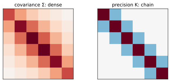
Marginal correlation everywhere, conditional dependence only along the chain.

Covariance selection: known graph

Sample \(x_1, \dots, x_N\), empirical covariance \(S\). Log-likelihood up to constants:

\[ \ell(K) = \frac N2 \big(\log\det K - \operatorname{tr}(S K)\big), \qquad \nabla_K \ell \propto K^{-1} - S \]

Graphical lasso: unknown graph

The graphical lasso penalises the \(\ell_1\) norm of the precision matrix to obtain a sparse estimate.

\[ \hat K_\lambda = \arg\min_{K \succ 0}\; -\log\det K + \operatorname{tr}(S K) + \lambda \sum_{s \neq t} |K_{st}| \]

• \(\lambda\) large → sparse graph
• Defined even for \(p > N\)
• Friedman, Hastie & Tibshirani (2008): block coordinate descent

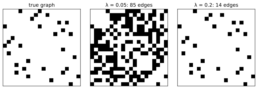
Graphical lasso on simulated data

Choice of \(\lambda\): cross-validation, StARS, BIC.

Graph learned: conditional dependences, not causal directions.

Structure learning

Structure learning: goals and obstacle

• Knowledge discovery: graph topology (gene networks, signalling pathways)
• Density estimation: fully specified model
• Obstacle: super-exponential number of DAGs

\(p\)	2	3	4	5	10
DAGs	3	25	543	29 281	\(4.2 \times 10^{18}\)

Robinson (1973). Structure learning of DAGs: NP-hard (Chickering, 1996).

Three families of methods

Family	Principle	Output
constraint-based	conditional independence tests	CPDAG (PC, FCI)
score-based	score optimisation over graphs	DAG or CPDAG (hill climbing, GES)
functional	restricted SCM class	DAG (LiNGAM, ANM)

Constraint-based learning: the PC algorithm

Assumptions

• Causal Markov: d-separation ⇒ independence
• Faithfulness: independence ⇒ d-separation
• Causal sufficiency: no unobserved common cause
• Reliable conditional independence tests

Key fact \(i\) and \(j\) non-adjacent in \(G\) iff some set \(S\) makes them independent: \(X_i \perp X_j \mid X_S\).

Conditional independence tests

• Gaussian: partial correlation, Fisher \(z\) transform

\[ z = \tfrac12 \log\frac{1 + \hat\rho_{ij \cdot S}}{1 - \hat\rho_{ij \cdot S}}\, \sqrt{N - |S| - 3} \;\approx\; \mathcal N(0, 1) \text{ under } H_0 \]

• Discrete: \(\chi^2\) or \(G^2\) test on contingency tables
• Non-linear: kernel tests (KCI)
• Level \(\alpha\): sparsity knob

PC step 1: skeleton

1. Start: complete undirected graph
2. For \(\ell = 0, 1, 2, \dots\): for each edge \(i - j\), test \(X_i \perp X_j \mid X_S\) for \(S \subseteq adj(i) \setminus \{j\}\), \(|S| = \ell\)
3. Independence accepted → edge removed, \(\operatorname{sepset}(i, j) = S\)
4. Stop when no node has more than \(\ell\) neighbours

Sparse graph → small conditioning sets → polynomial cost.

PC step 2: v-structures

For each triple \(i - k - j\) with \(i\) and \(j\) non-adjacent:

\[ k \notin \operatorname{sepset}(i, j) \;\Longrightarrow\; i \to k \leftarrow j \]

• \(k\) in the separating set: chain or fork, no orientation
• \(k\) absent: collider, the only structure making \(i, j\) dependent given \(k\)

PC step 3: Meek rules

Orientation propagation, no new v-structure, no cycle:

• R1: \(a \to b - c\), \(a, c\) non-adjacent → \(b \to c\)
• R2: \(a \to b \to c\) and \(a - c\) → \(a \to c\)
• R3: two chains \(a - c_1 \to b\), \(a - c_2 \to b\), \(c_1, c_2\) non-adjacent, \(a - b\) → \(a \to b\)

PC on an example

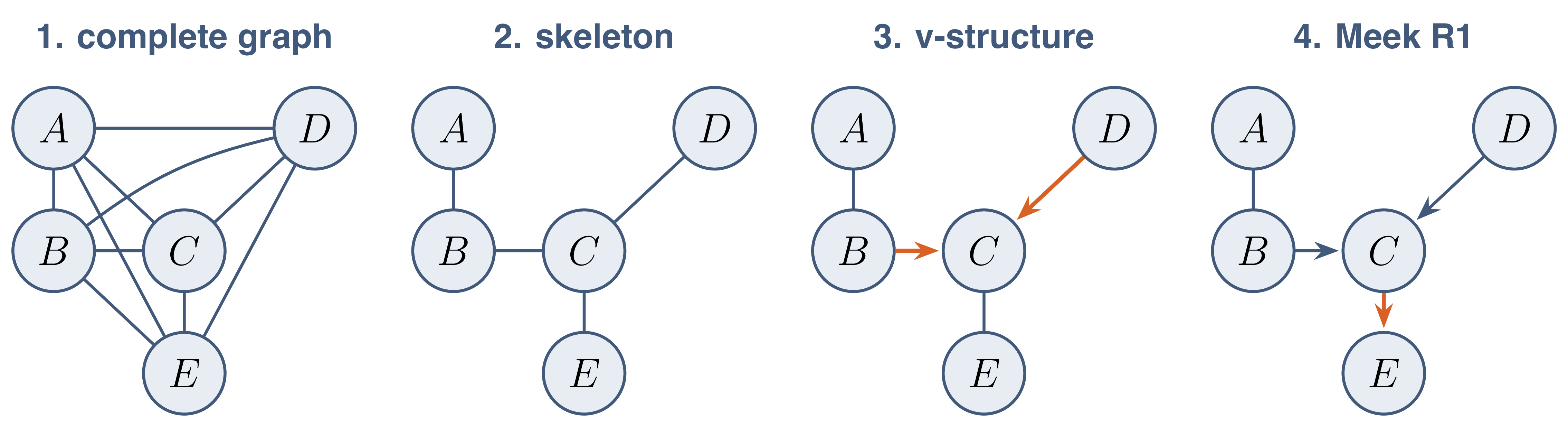
• Removed: \(A - C\) (\(S = \{B\}\)), \(A - D\), \(B - D\) (\(S = \emptyset\)), \(A - E, B - E, D - E\) (\(S = \{C\}\))
• \(C \notin \operatorname{sepset}(B, D) = \emptyset\) → \(B \to C \leftarrow D\)
• R1 → \(C \to E\); \(A - B\) unoriented

PC with causal-learn

import numpy as np
from causallearn.search.ConstraintBased.PC import pc
rng = np.random.default_rng(0); N = 2000
A = rng.standard_normal(N); D = rng.standard_normal(N)
B = 0.8 * A + rng.standard_normal(N)
C = 0.7 * B - 0.6 * D + rng.standard_normal(N)
E = 0.9 * C + rng.standard_normal(N)
cg = pc(np.c_[A, B, C, D, E], alpha=0.01, indep_test="fisherz",
        node_names=list("ABCDE"), show_progress=False)
print(cg.G)

Graph Nodes:
A;B;C;D;E

Graph Edges:
1. A --- B
2. B --> C
3. D --> C
4. C --> E

PC: properties and limits

• Consistent under the assumptions, oracle tests → exact CPDAG
• Test errors propagate; result depends on variable order → PC-stable
• Hidden confounders: FCI (partial ancestral graphs)
• Near-violations of faithfulness: unstable orientations

Evaluation of learned graphs

Structural Hamming distance

The structural Hamming distance counts the elementary edge operations turning the estimated graph into the true one.

\[ \operatorname{SHD}(\hat G, G) = \#\{\text{edge additions}\} + \#\{\text{deletions}\} + \#\{\text{reversals}\} \]

• Compared on CPDAGs when only the class is identifiable
• Complements: precision and recall on the skeleton, on arrowheads