Causality and directed graphical models

M2 GENIOMHE — Session 1

Christophe Ambroise

M2 GENIOMHE — Université d’Évry

Course overview

Three sessions

# Lecture Tutorial
1 Causality, DAGs, d-separation Simpson, d-separation, sprinkler network
2 Biological networks: GGM, PC algorithm graphical lasso and PC on cytometry data
3 Interventions, Mendelian randomisation, LiNGAM adjustment, MR, causal order of RNA editing

References

  • J. Pearl, M. Glymour, N. Jewell, Causal Inference in Statistics: a Primer (2016)
  • K. Murphy, Machine Learning: a Probabilistic Perspective (2012), ch. 10, 19, 26
  • S. Shimizu, Statistical Causal Discovery: LiNGAM Approach (2022)

Why causality

Cause and effect

Cause: that which produces or modifies an effect.

  • Aristotle (384-322 BC): knowledge of a thing = grasp of its why
  • Hume (1711-1776): Causality stems from habit or mental expectation, built over repeated experience
  • Science: temporal order + mechanism, e.g. \(\dfrac{dY}{dt} = f(X, Y, t)\)

Three statistical views of causality

  • Dependence: \(P(Y \mid X = x) \neq P(Y)\)
  • Prediction (Granger): past of \(X\) → better forecast of \(Y\)
  • Intervention (Pearl): forced change of \(X\) → change in \(Y\)

Intervention view \(X\) causes \(Y\) when the distribution of \(Y\) under a forced value of \(X\) depends on that value.

\[ \exists\, x \neq x' : \quad P\big(Y \mid do(X = x)\big) \neq P\big(Y \mid do(X = x')\big) \]

Ladder of causation

Rung Activity Typical question Quantity
1. Association seeing patients with \(X\): recovery? \(P(y \mid x)\)
2. Intervention doing recovery if \(X\) imposed? \(P(y \mid do(x))\)
3. Counterfactual imagining this patient, without \(X\)? \(P(y_{x'} \mid x, y)\)

Each rung: more assumptions, more structure.

Pearl & Mackenzie, The Book of Why (2018).

Simpson’s paradox: kidney stones

Stone size Treatment Recovered Total Rate
Small New 81 87 93 %
Small Standard 234 270 87 %
Large New 192 263 73 %
Large Standard 55 80 69 %
All New 273 350 78 %
All Standard 289 350 83 %

New drug: better in each stratum, worse overall.

Charig et al. (1986), BMJ.

Mechanism of the reversal

  • New drug: mostly large stones (263 / 350)
  • Large stones: harder to treat, whatever the drug
  • Aggregate rate = mixture with different weights

\[ \begin{aligned} P(R \mid T = \text{new}) &= \textstyle\sum_s P(R \mid T = \text{new}, s)\, P(s \mid T = \text{new}) \\ &\neq \textstyle\sum_s P(R \mid T = \text{new}, s)\, P(s) \end{aligned} \]

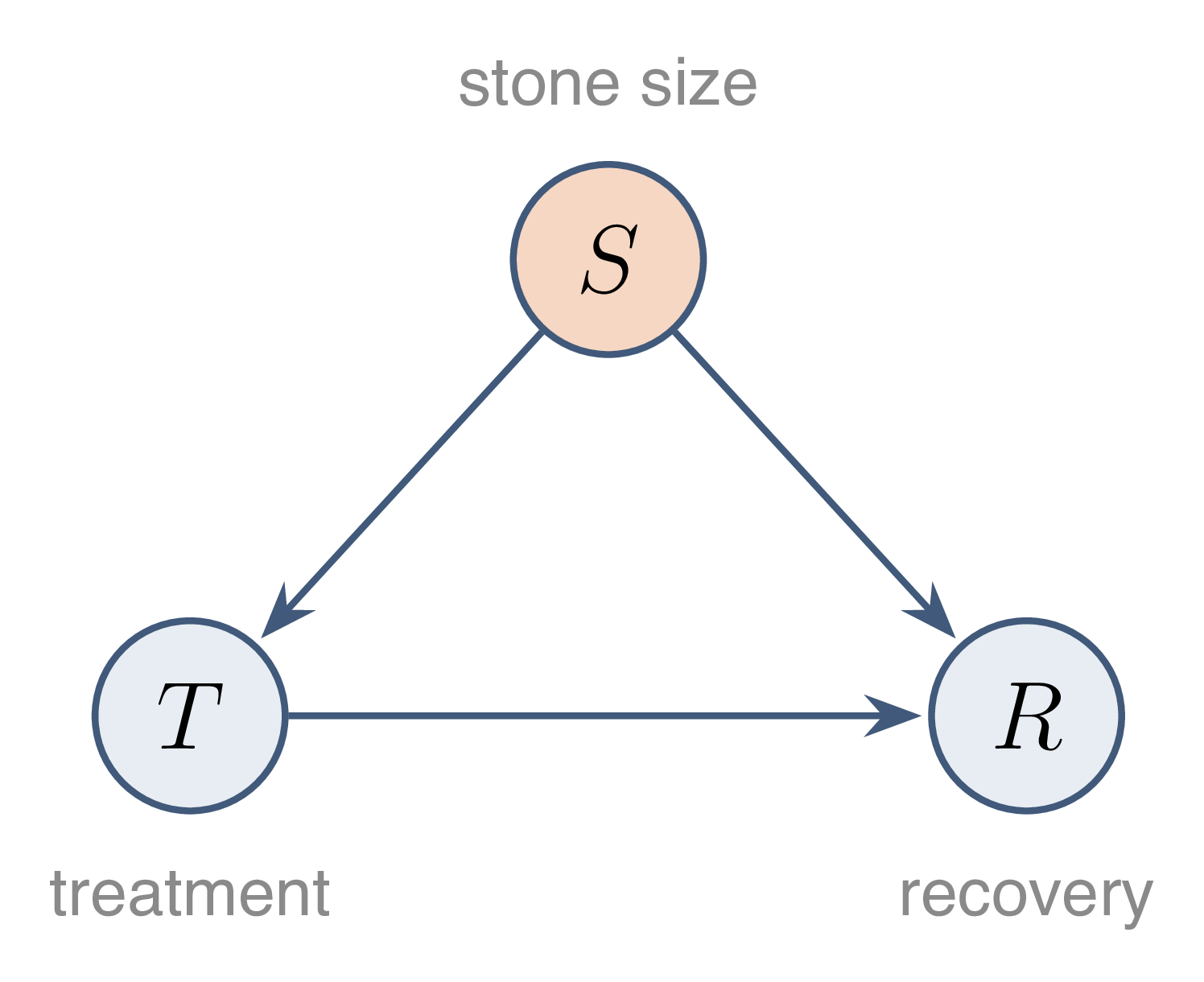
Causal graph of the paradox

  • \(S\) (stone size): common cause of \(T\) and \(R\) → confounder
  • Right comparison: within strata of \(S\)

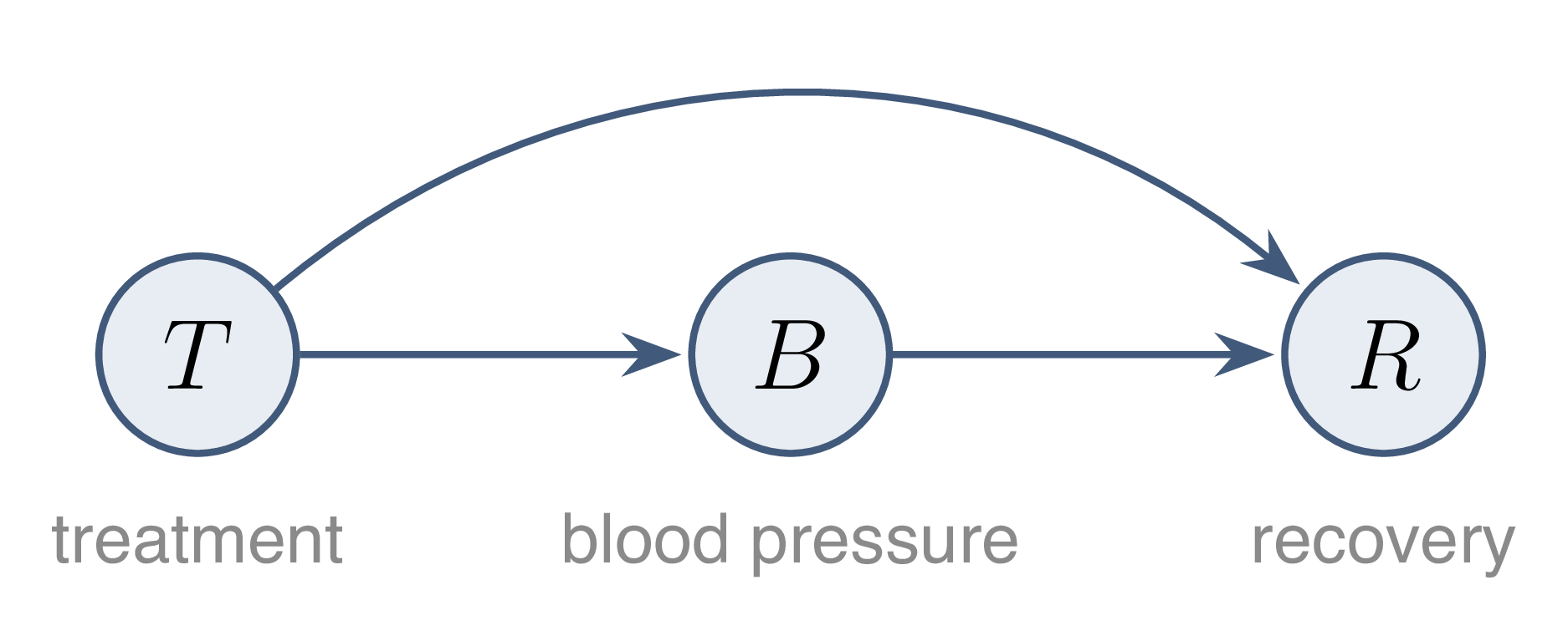
Same table, another graph

  • \(B\): post-treatment variable (e.g. blood pressure), mediator
  • Stratification on \(B\): part of the effect removed → aggregate rate correct

Lesson Same numbers, opposite conclusions: the decision depends on the causal graph, not on the data alone.

Directed graphical models

Joint distribution: size problem

  • Many correlated variables: genes, pixels, words
  • Goal: compact representation of \(p(x_1, \dots, x_V)\)

Chain rule, any ordering of the variables:

\[ p(x_{1:V}) = p(x_1)\, p(x_2 \mid x_1)\, p(x_3 \mid x_1, x_2) \cdots p(x_V \mid x_{1:V-1}) \]

\(K\) states per variable → \(O(K^V)\) parameters.

Conditional independence

\(X\) is conditionally independent of \(Y\) given \(Z\) when, once \(Z\) is known, \(Y\) brings no further information on \(X\).

\[ X \perp Y \mid Z \iff p(x, y \mid z) = p(x \mid z)\, p(y \mid z) \quad \forall\, x, y, z \text{ with } p(z) > 0 \]

Graphical model

  • Node = random variable
  • Missing edge = conditional independence assumption
  • Graph types: directed (DAG), undirected, mixed

Graphical model Joint distribution in factorised form, the factorisation being encoded by a graph.

Graph vocabulary

Term Definition
parents \(pa(s)\) \(\{t : t \to s\}\)
children \(ch(s)\) \(\{t : s \to t\}\)
ancestors \(an(s)\) nodes with a directed path to \(s\)
descendants \(de(s)\) nodes reached from \(s\) by a directed path
non-descendants \(nd(s)\) \(V \setminus (de(s) \cup \{s\})\)
root / leaf no parent / no child

Directed acyclic graph

A DAG is a directed graph without directed cycle; its nodes then admit a topological order, parents before children.

\[ G \text{ acyclic} \iff \exists\, \pi \text{ permutation of } V : \quad s \to t \in E \Rightarrow \pi(s) < \pi(t) \]

  • Order not unique in general
  • Construction: repeated removal of roots

DAG factorisation

A distribution factorises according to a DAG \(G\) when each variable depends only on its parents.

\[ p(x_1, \dots, x_V) = \prod_{t=1}^{V} p\big(x_t \mid x_{pa(t)}\big) \]

Bayesian network DAG \(G\) + one conditional distribution \(p(x_t \mid x_{pa(t)})\) per node (CPD).

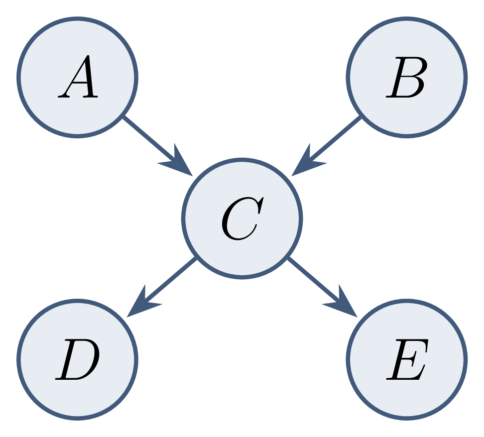
Parameter count: example

Binary variables:

Factor Parameters
\(p(a)\), \(p(b)\) \(1 + 1\)
\(p(c \mid a, b)\) \(4\)
\(p(d \mid c)\), \(p(e \mid c)\) \(2 + 2\)
DAG 10
full joint \(2^5 - 1 = 31\)

Classical examples

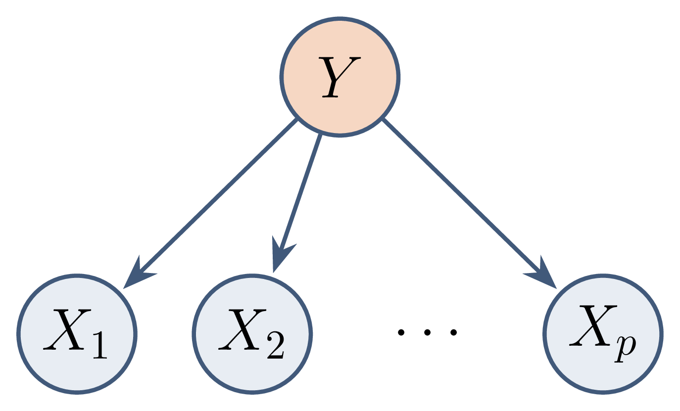
Naive Bayes classifier

\[ p(y, x) = p(y) \prod_{j=1}^{p} p(x_j \mid y) \]

Features: independent given the class.

Gaussian Bayesian network

Each variable is a linear function of its parents plus an independent Gaussian noise.

\[ p(x_t \mid x_{pa(t)}) = \mathcal N\big(x_t \;\big|\; \mu_t + \textstyle\sum_{s \in pa(t)} w_{ts}(x_s - \mu_s),\ \sigma_t^2\big) \]

Equivalent structural equations, \(z_t \sim \mathcal N(0, 1)\) independent:

\[ x_t = \mu_t + \textstyle\sum_{s \in pa(t)} w_{ts}(x_s - \mu_s) + \sigma_t z_t \]

Linear structural equation model

Matrix form, \(W = (w_{ts})\), \(S = \operatorname{diag}(\sigma_t)\), \(e = S z\):

\[ x - \mu = W (x - \mu) + e \]

  • Topological order → \(W\) strictly lower triangular → \(I - W\) invertible
  • \(x - \mu = (I - W)^{-1} e\): linear mixture of independent noises

Covariance of a Gaussian Bayesian network \[ \Sigma = (I - W)^{-1}\, S^2\, (I - W)^{-\top}, \qquad x \sim \mathcal N(\mu, \Sigma) \]

Simulation check

import numpy as np
rng = np.random.default_rng(0)
W = np.array([[0, 0, 0],      # x1 = e1
              [0.8, 0, 0],    # x2 = 0.8 x1 + e2
              [0, -0.5, 0]])  # x3 = -0.5 x2 + e3
S = np.diag([1.0, 0.6, 0.3])
U = np.linalg.inv(np.eye(3) - W)
Sigma = U @ S**2 @ U.T
X = (U @ S @ rng.standard_normal((3, 100_000))).T
print(np.round(Sigma, 3)); print(np.round(np.cov(X.T), 3))
[[ 1.    0.8  -0.4 ]
 [ 0.8   1.   -0.5 ]
 [-0.4  -0.5   0.34]]
[[ 1.     0.801 -0.401]
 [ 0.801  1.004 -0.502]
 [-0.401 -0.502  0.341]]

Two DAGs, one covariance

  • \(X_2 = w X_1 + e_2\) and \(X_1 = w' X_2 + e_1'\): both Gaussian, same \(\Sigma\) for suitable \(w'\)
  • Gaussian observational data: direction not recoverable

Identifiability DAG factorisation: a statistical model; the arrow direction is not always identifiable from \(p\) alone.

Conditional independence in DAGs

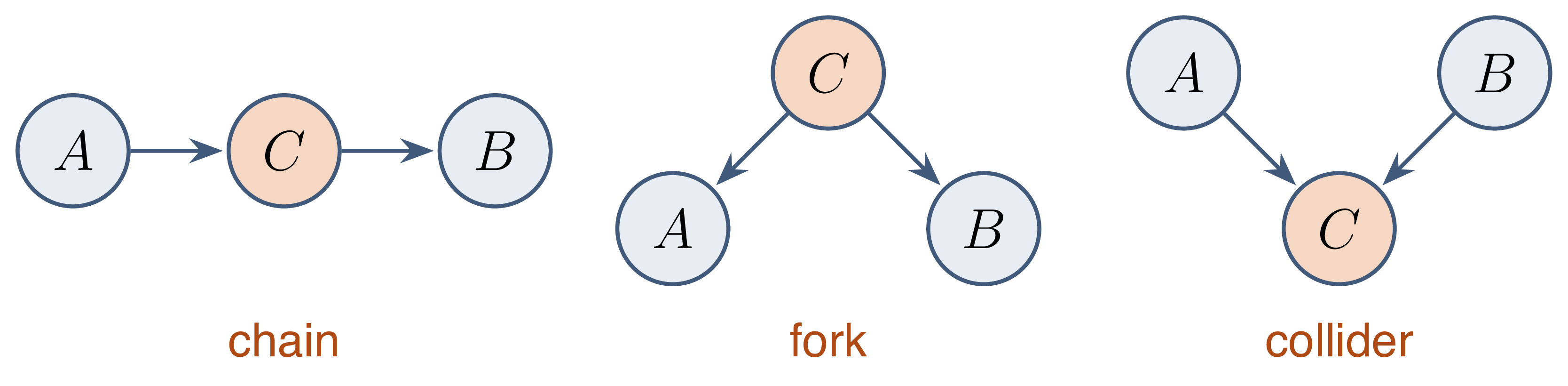
Three elementary structures

Structure Marginal Given \(C\)
chain \(A \to C \to B\) \(A \not\perp B\) \(A \perp B \mid C\)
fork \(A \leftarrow C \to B\) \(A \not\perp B\) \(A \perp B \mid C\)
collider \(A \to C \leftarrow B\) \(A \perp B\) \(A \not\perp B \mid C\)

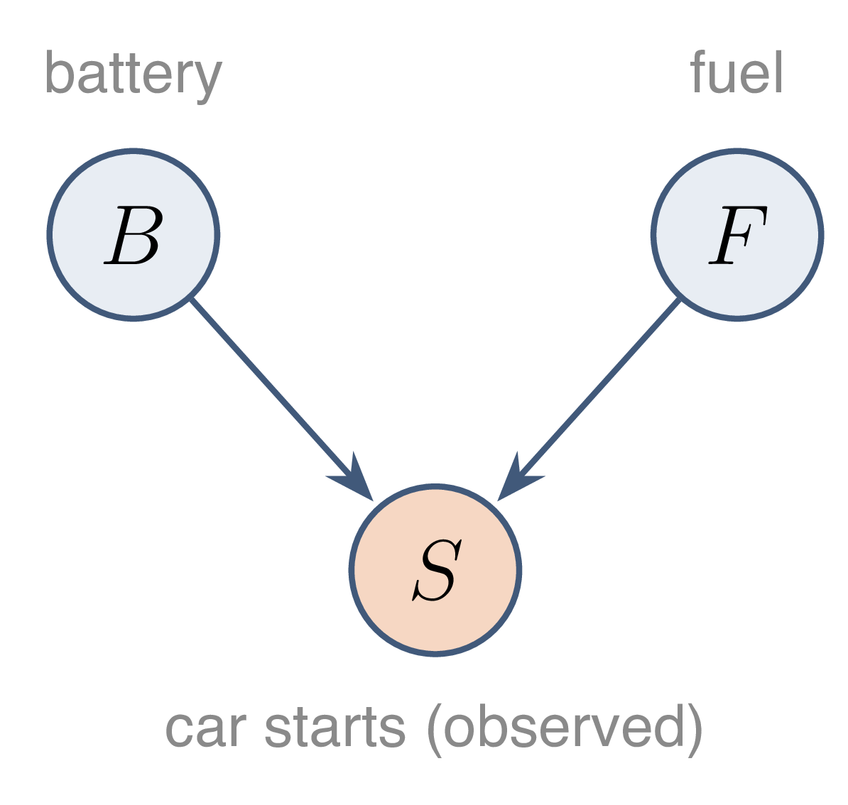
Explaining away

  • Battery state \(\perp\) fuel level
  • Car not starting + battery fine → empty tank
  • Two independent causes, dependent given the common effect

Pearl (1988), Probabilistic Reasoning in Intelligent Systems.

Selection on a collider: Berkson bias

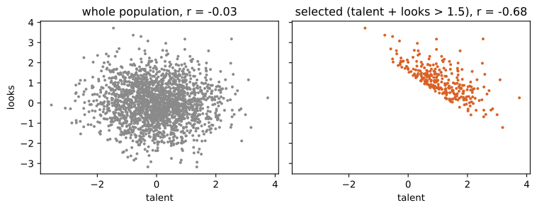
Selection = conditioning on a collider → spurious negative correlation.

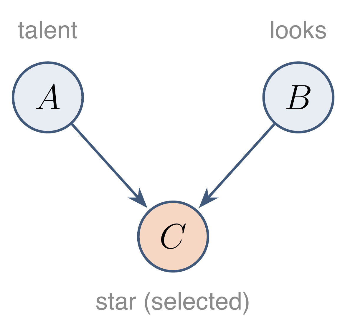
Berkson bias as a collider

  • \(A\), \(B\): independent causes of \(C\)
  • Path blocked: \(A \perp B\)
  • Selection on \(C\): \(A \not\perp B \mid C\)
  • Low-talent star → high looks: \(r < 0\)

Selecting stars conditions on the collider and couples the two causes.

\[ p(a, b \mid C = 1) \propto p(a)\, p(b)\, \mathbb{1}\{a + b > 1.5\} \]

Blocked path

A path between two nodes is blocked by a set \(E\) when it contains at least one of the following nodes \(m\).

\[ \begin{aligned} &\text{chain } s \to m \to t \text{ or fork } s \leftarrow m \to t, &&\text{with } m \in E \\ &\text{collider } s \to m \leftarrow t, &&\text{with } (\{m\} \cup de(m)) \cap E = \emptyset \end{aligned} \]

Path not blocked = active: carries dependence.

d-separation

Two sets \(A\) and \(B\) are d-separated by \(E\) when every path between a node of \(A\) and a node of \(B\) is blocked by \(E\).

\[ A \perp_G B \mid E \iff \forall\, \text{path } a \leadsto b,\ a \in A,\ b \in B: \text{ path blocked by } E \]

  • Independence: all paths blocked
  • Dependence: one active path suffices

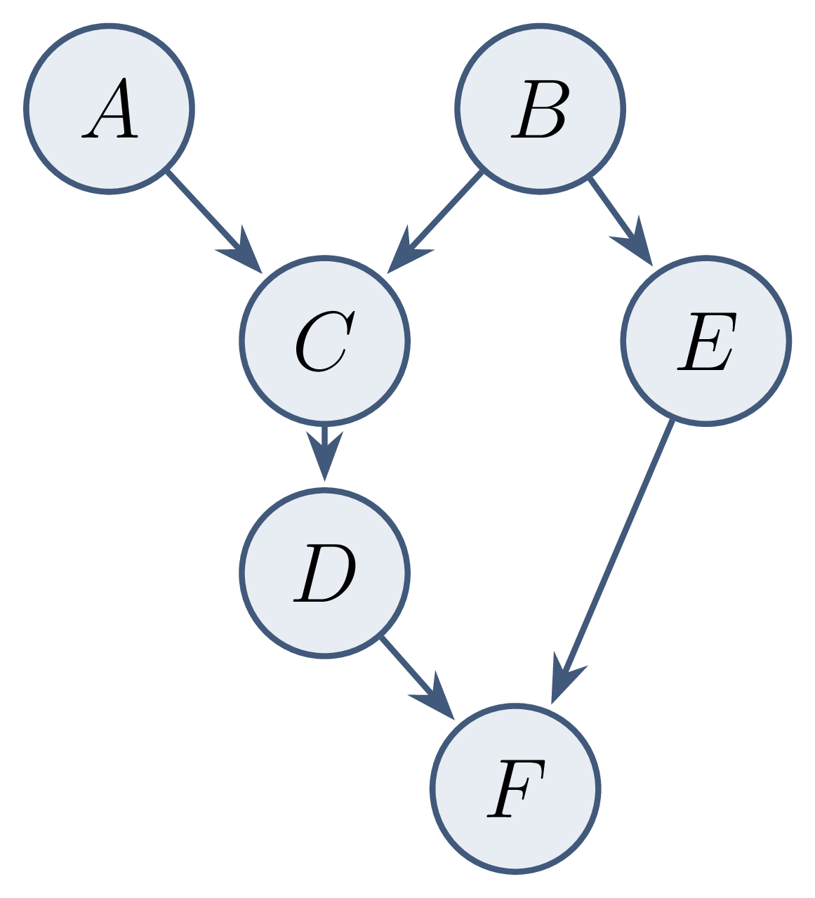
d-separation: worked example

Query Answer
\(A \perp B\) yes
\(A \perp B \mid F\) no: \(C\) opened via \(F\)
\(A \perp E \mid C\) no: \(A \to C \leftarrow B \to E\)
\(A \perp E \mid \{B, C\}\) yes
\(D \perp E \mid \{B, C\}\) yes

Global Markov property

If \(p\) factorises according to \(G\), every d-separation in \(G\) is a conditional independence of \(p\).

\[ p(x) = \prod_t p(x_t \mid x_{pa(t)}) \;\Longrightarrow\; \big(A \perp_G B \mid E \Rightarrow X_A \perp X_B \mid X_E\big) \]

  • Converse false in general: extra independences possible
  • Graph = safe proxy for \(p\)

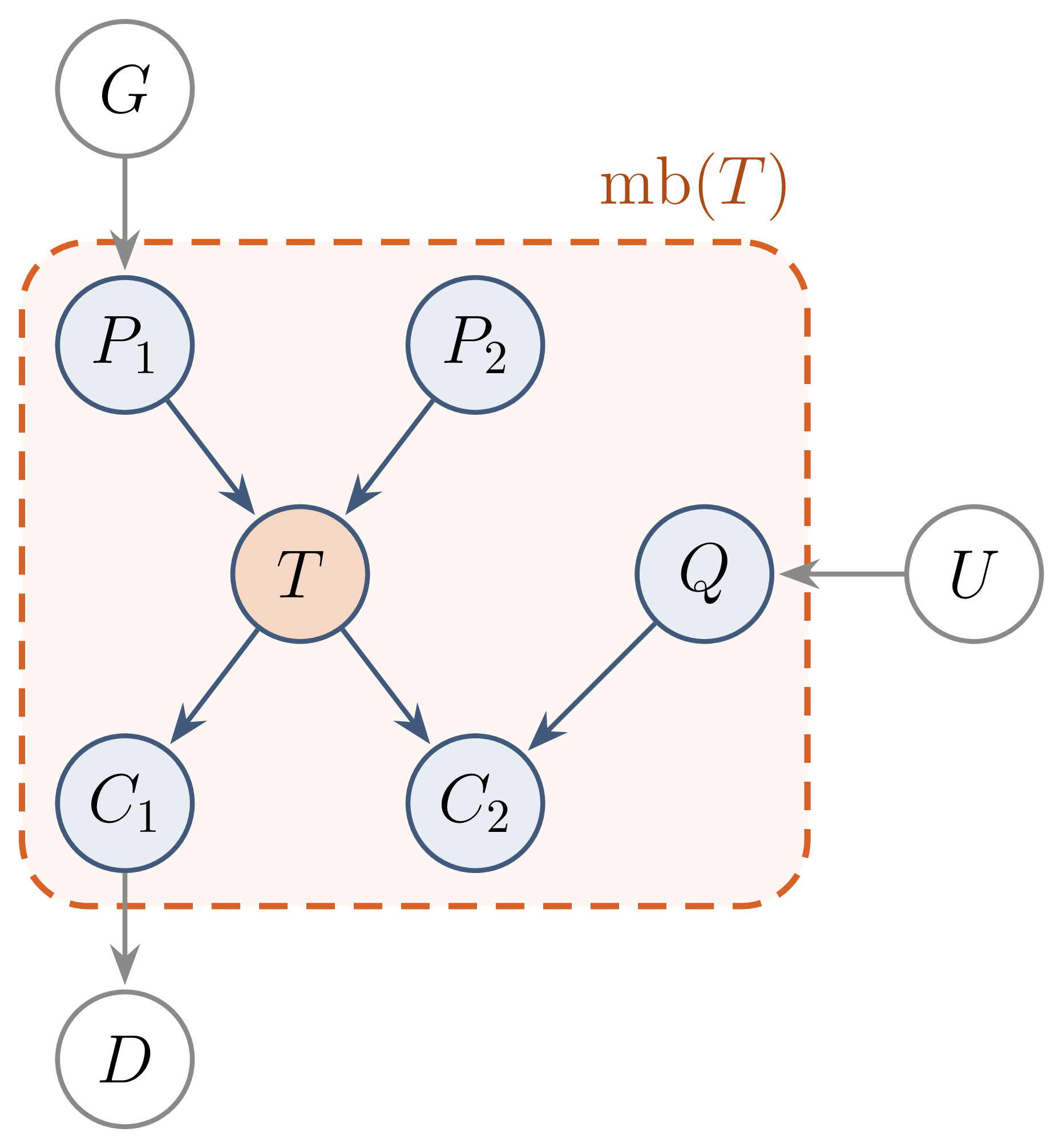
Markov blanket

In a DAG, the parents, children and co-parents of a node make it independent of all other nodes: this set is its Markov blanket.

\[ mb(t) = \Big(pa(t) \cup ch(t) \cup \textstyle\bigcup_{c \in ch(t)} pa(c)\Big) \setminus \{t\}, \qquad X_t \perp X_{V \setminus (mb(t) \cup \{t\})} \mid X_{mb(t)} \]

Markov blanket: role of each part

  • Parents: block paths towards non-descendants
  • Children: block paths towards descendants
  • Conditioning on children → colliders opened → co-parents needed
  • Use: feature selection, Gibbs sampling, local structure learning

Markov equivalence

Faithfulness

A distribution is faithful to \(G\) when its conditional independences are exactly the d-separations of \(G\).

\[ X_A \perp X_B \mid X_E \iff A \perp_G B \mid E \]

Three nodes, two equivalence classes

  • Chain, reverse chain, fork: same independence \(A \perp B \mid C\)
  • Collider: \(A \perp B\), alone in its class

Markov equivalence

Two DAGs are Markov equivalent when they encode the same d-separations.

\[ G_1 \sim G_2 \iff I(G_1) = I(G_2) \]

Verma–Pearl theorem (1990) Two DAGs are Markov equivalent if and only if they have the same skeleton and the same v-structures.

v-structure: \(a \to c \leftarrow b\) with \(a\) and \(b\) non-adjacent.

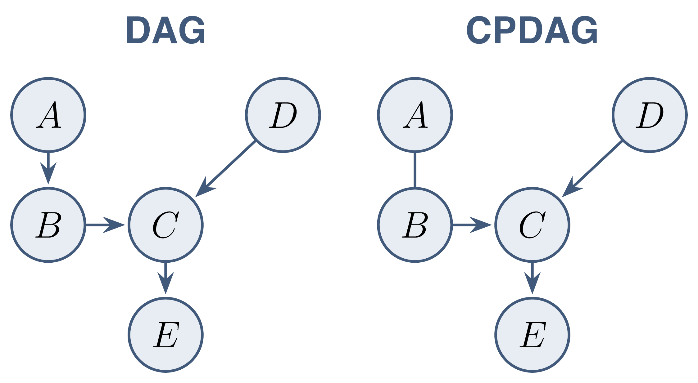
CPDAG: representation of a class

CPDAG (completed partially directed acyclic graph), or essential graph: a single graph standing for a whole Markov equivalence class, i.e. all DAGs encoding the same conditional independences.

  • Directed edge: same orientation in every DAG of the class
  • Undirected edge: orientation varies within the class
  • \(B \to C \leftarrow D\): v-structure; \(C \to E\): forced, else new v-structure

Limit of observational data

  • Observational data + faithfulness → CPDAG at best
  • Gaussian linear models: no further information
  • Orientation of undirected edges: extra ingredients

Beyond the equivalence class Interventions, temporal order, or distributional assumptions (non-Gaussian noise, non-linear mechanisms).