Projection orthogonale et moindres carrés
Cours 7 — Algèbre linéaire et analyse de données
L3 GBI — Université d’Évry
Résoudre l’insoluble
Trop d’équations
Une expérience : \(50\) mesures, \(2\) paramètres à estimer.
\(50\) équations, \(2\) inconnues.
\[\operatorname{rg}(A) \leqslant 2 < 50 \ \Longrightarrow \ \operatorname{Im}(A) \ \text{est un plan de } \mathbb{R}^{50}\]
Presque toujours incompatible
\(\mathbf{b} \in \operatorname{Im}(A)\) : une coïncidence.
Le bruit de mesure suffit à l’empêcher.
Changement de question À défaut de résoudre \(A\mathbf{x} = \mathbf{b}\), chercher \(\mathbf{x}\) rendant \(A\mathbf{x}\) aussi proche que possible de \(\mathbf{b}\).
Le critère
\[\min_{\mathbf{x} \in \mathbb{R}^n} \ \|A\mathbf{x} - \mathbf{b}\|\]
La norme du cours 6. Minimiser une distance.
\(A\mathbf{x}\) parcourt \(\operatorname{Im}(A)\) : un problème de géométrie.
Projection sur une droite
Le cas le plus simple
\(D = \operatorname{Vect}(\mathbf{u})\), avec \(\|\mathbf{u}\| = 1\).
Quel point de \(D\) est le plus proche de \(\mathbf{x}\) ?
Construction
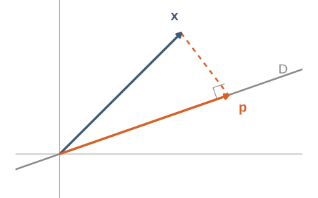
Figure 1
Le pied de la perpendiculaire.
Formule
\[\mathbf{p} = \langle \mathbf{x}, \mathbf{u} \rangle \, \mathbf{u} \qquad (\|\mathbf{u}\| = 1)\]
Sans normalisation :
\[\mathbf{p} = \frac{\langle \mathbf{x}, \mathbf{u} \rangle}{\|\mathbf{u}\|^2} \, \mathbf{u}\]
Le résidu
\(\mathbf{r} = \mathbf{x} - \mathbf{p}\).
\[\langle \mathbf{r}, \mathbf{u} \rangle = \langle \mathbf{x}, \mathbf{u} \rangle - \langle \mathbf{x}, \mathbf{u} \rangle \|\mathbf{u}\|^2 = 0\]
Caractérisation \(\mathbf{p}\) est la projection de \(\mathbf{x}\) sur \(D\) \(\iff\) \(\mathbf{p} \in D\) et \(\mathbf{x} - \mathbf{p} \perp D\).
Exemple numérique
\(\mathbf{x} = (1,\, 2,\, 3)\), \(D = \operatorname{Vect}(\mathbf{1})\) avec \(\mathbf{1} = (1,1,1)\).
\[\mathbf{p} = \frac{\langle \mathbf{x}, \mathbf{1} \rangle}{\|\mathbf{1}\|^2}\,\mathbf{1} = \frac{6}{3}\,\mathbf{1} = (2,\, 2,\, 2)\]
\[\mathbf{r} = \mathbf{x} - \mathbf{p} = (-1,\, 0,\, 1), \qquad \langle \mathbf{r}, \mathbf{1} \rangle = 0\]
Le centrage est une projection
\(\mathbf{p} = (2,2,2) = \bar{x}\,\mathbf{1}\), et \(\mathbf{r} = \tilde{\mathbf{x}}\).
Reformulation Centrer une variable, c’est la projeter sur l’orthogonal de \(\mathbf{1}\). \[\tilde{\mathbf{x}} = \mathbf{x} - \operatorname{proj}_{\operatorname{Vect}(\mathbf{1})}(\mathbf{x})\]
La moyenne apparaît comme une coordonnée, pas comme une convention.
Projection sur un sous-espace
Théorème de la projection
Théorème Soit \(F\) un sous-espace de \(\mathbb{R}^n\) et \(\mathbf{x} \in \mathbb{R}^n\). Il existe un unique \(\mathbf{p} \in F\) tel que \(\mathbf{x} - \mathbf{p} \perp F\).
Notation : \(\mathbf{p} = \operatorname{proj}_F(\mathbf{x})\).
Orthogonal à tout \(F\)
Il suffit de tester sur une famille génératrice.
\[\mathbf{r} \perp F \iff \forall i, \ \langle \mathbf{r}, \mathbf{v}_i \rangle = 0\]
Un nombre fini de conditions.
Sous-espace orthogonal
\[F^{\perp} = \{\, \mathbf{y} \in \mathbb{R}^n \mid \forall \mathbf{v} \in F, \ \langle \mathbf{y}, \mathbf{v} \rangle = 0 \,\}\]
Un sous-espace vectoriel, lui aussi.
Le résidu d’une projection sur \(F\) vit dans \(F^{\perp}\).
Dimensions complémentaires
Théorème \[\dim F + \dim F^{\perp} = n\]
Tout vecteur se décompose de façon unique en une part dans \(F\) et une part dans \(F^{\perp}\).
\[\mathbb{R}^n = F \oplus F^{\perp}\]
La meilleure approximation
Théorème \[\forall \mathbf{y} \in F, \ \mathbf{y} \neq \mathbf{p}, \qquad \|\mathbf{x} - \mathbf{p}\| < \|\mathbf{x} - \mathbf{y}\|\]
La projection est le point de \(F\) le plus proche de \(\mathbf{x}\).
Démonstration
\(\mathbf{x} - \mathbf{y} = (\mathbf{x} - \mathbf{p}) + (\mathbf{p} - \mathbf{y})\), deux termes orthogonaux.
\[\|\mathbf{x} - \mathbf{y}\|^2 = \|\mathbf{x} - \mathbf{p}\|^2 + \|\mathbf{p} - \mathbf{y}\|^2\]
Pythagore. Le second terme est nul si et seulement si \(\mathbf{y} = \mathbf{p}\).
Formule en base orthonormée
\((\mathbf{u}_1, \dots, \mathbf{u}_k)\) base orthonormée de \(F\) :
\[\operatorname{proj}_F(\mathbf{x}) = \sum_{i=1}^{k} \langle \mathbf{x}, \mathbf{u}_i \rangle \, \mathbf{u}_i\]
La formule des coordonnées du cours 6, tronquée aux \(k\) premiers termes.
Une décomposition
\[\mathbf{x} = \underbrace{\operatorname{proj}_F(\mathbf{x})}_{\in F} + \underbrace{\mathbf{r}}_{\perp F}, \qquad \|\mathbf{x}\|^2 = \|\operatorname{proj}_F(\mathbf{x})\|^2 + \|\mathbf{r}\|^2\]
À retenir pour l’ACP La norme se partage entre la part retenue et la part perdue. Projeter : choisir la part gardée.
Moindres carrés
Traduction du problème
\(A\mathbf{x}\) parcourt \(\operatorname{Im}(A)\) quand \(\mathbf{x}\) parcourt \(\mathbb{R}^n\).
\[\min_{\mathbf{x}} \|A\mathbf{x} - \mathbf{b}\| \ \Longleftrightarrow \ A\hat{\mathbf{x}} = \operatorname{proj}_{\operatorname{Im}(A)}(\mathbf{b})\]
Le minimum est atteint : la projection existe toujours.
Le résidu, encore
\(\hat{\mathbf{x}}\) optimal \(\iff\) \(\mathbf{b} - A\hat{\mathbf{x}} \perp \operatorname{Im}(A)\).
\(\operatorname{Im}(A)\) est engendré par les colonnes de \(A\) :
\[\forall j, \ \langle \mathbf{a}_j, \mathbf{b} - A\hat{\mathbf{x}} \rangle = 0 \ \Longleftrightarrow \ A^{\intercal}(\mathbf{b} - A\hat{\mathbf{x}}) = \mathbf{0}\]
Équations normales
Résultat central \[A^{\intercal}A\,\hat{\mathbf{x}} = A^{\intercal}\mathbf{b}\]
Un système \(n \times n\), toujours compatible.
Le pivot de Gauss, une dernière fois.
Unicité
\[\text{colonnes de } A \ \text{libres} \iff A^{\intercal}A \ \text{inversible} \ \Longrightarrow \ \hat{\mathbf{x}} = (A^{\intercal}A)^{-1}A^{\intercal}\mathbf{b}\]
Colonnes liées : une infinité de \(\hat{\mathbf{x}}\), mais une seule projection \(A\hat{\mathbf{x}}\).
Noyaux de \(A\) et de \(A^{\intercal}A\)
\[A^{\intercal}A\mathbf{x} = \mathbf{0} \ \Longrightarrow \ \mathbf{x}^{\intercal}A^{\intercal}A\mathbf{x} = \|A\mathbf{x}\|^2 = 0 \ \Longrightarrow \ A\mathbf{x} = \mathbf{0}\]
Conséquence \(\operatorname{Ker}(A^{\intercal}A) = \operatorname{Ker}(A)\), donc \(A^{\intercal}A\) est inversible exactement quand les colonnes de \(A\) sont libres.
Matrice de projection
Colonnes de \(A\) libres :
\[\operatorname{proj}_{\operatorname{Im}(A)}(\mathbf{b}) = A\hat{\mathbf{x}} = \underbrace{A(A^{\intercal}A)^{-1}A^{\intercal}}_{H}\ \mathbf{b}\]
Une matrice \(H\), qui projette tout vecteur sur \(\operatorname{Im}(A)\).
Deux propriétés
\[H^2 = H, \qquad H^{\intercal} = H\]
Projeter deux fois ne change rien : le résultat est déjà dans \(F\).
Réciproque Toute matrice vérifiant \(H^2 = H\) et \(H^{\intercal} = H\) est une matrice de projection orthogonale.
Le nom
\(\|A\mathbf{x} - \mathbf{b}\|^2 = \sum_{i=1}^{m} (\text{résidu}_i)^2\).
\[\min_{\mathbf{x}} \ \sum_{i=1}^{m} \bigl( b_i - (A\mathbf{x})_i \bigr)^2\]
Minimiser une somme de carrés : moindres carrés.
Régression linéaire
Le modèle
\(n\) couples \((x_i, y_i)\). Ajuster une droite :
\[y_i \approx \beta_0 + \beta_1 x_i\]
Deux inconnues, \(n\) équations.
Mise en matrice
\[ A = \begin{pmatrix} 1 & x_1 \\ 1 & x_2 \\ \vdots & \vdots \\ 1 & x_n \end{pmatrix}, \qquad \boldsymbol{\beta} = \begin{pmatrix} \beta_0 \\ \beta_1 \end{pmatrix}, \qquad \mathbf{y} = \begin{pmatrix} y_1 \\ \vdots \\ y_n \end{pmatrix} \]
La colonne de \(1\) porte l’ordonnée à l’origine.
Un jeu de données
\[ \mathbf{x} = (1,\, 2,\, 3,\, 4), \qquad \mathbf{y} = (2,\, 3,\, 5,\, 6) \]
\[A^{\intercal}A = \begin{pmatrix} 4 & 10 \\ 10 & 30 \end{pmatrix}, \qquad A^{\intercal}\mathbf{y} = \begin{pmatrix} 16 \\ 47 \end{pmatrix}\]
\[\hat{\beta}_0 = 0{,}5, \qquad \hat{\beta}_1 = 1{,}4\]
L’ajustement
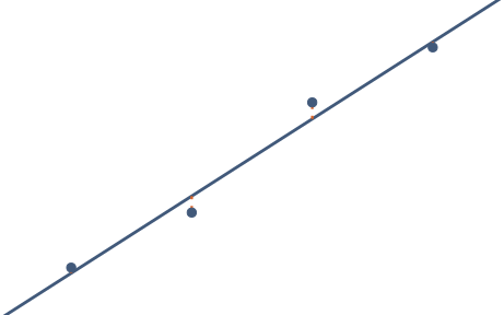
Figure 2
En pointillé : les résidus. Leur somme des carrés est minimale.
Lecture géométrique
\(\mathbf{y}\) vit dans \(\mathbb{R}^4\).
\(\operatorname{Im}(A)\) : un plan de \(\mathbb{R}^4\), engendré par \(\mathbf{1}\) et \(\mathbf{x}\).
Deux images d’un même calcul Sur le graphique : une droite ajustée à quatre points. Dans \(\mathbb{R}^4\) : un vecteur projeté sur un plan.
Le résidu est orthogonal
\[\langle \mathbf{1}, \mathbf{y} - A\hat{\boldsymbol{\beta}} \rangle = 0 \ \Longleftrightarrow \ \sum_i r_i = 0\]
\[\langle \mathbf{x}, \mathbf{y} - A\hat{\boldsymbol{\beta}} \rangle = 0 \ \Longleftrightarrow \ \sum_i x_i r_i = 0\]
Deux propriétés classiques de la régression : les équations normales, en clair.
Valeurs ajustées
\[\hat{\mathbf{y}} = H\mathbf{y}, \qquad \mathbf{r} = (I_n - H)\,\mathbf{y}\]
\(H\) produit les valeurs prédites, \(I_n - H\) les résidus.
Deux projections complémentaires, sur \(\operatorname{Im}(A)\) et sur \(\operatorname{Im}(A)^{\perp}\).
Au-delà de la droite
Ajuster une parabole \(y_i \approx \beta_0 + \beta_1 x_i + \beta_2 x_i^2\) :
\[ A = \begin{pmatrix} 1 & x_1 & x_1^2 \\ \vdots & \vdots & \vdots \\ 1 & x_n & x_n^2 \end{pmatrix} \]
Linéaire en quoi ? Le modèle est linéaire en les paramètres \(\beta_j\), non en \(x\). Les équations normales s’appliquent sans changement.
Qualité de l’ajustement
\[\|\tilde{\mathbf{y}}\|^2 = \underbrace{\|\hat{\mathbf{y}} - \bar{y}\mathbf{1}\|^2}_{\text{expliqué}} + \underbrace{\|\mathbf{r}\|^2}_{\text{résiduel}}\]
Le coefficient \(R^2\) \[R^2 = \frac{\text{expliqué}}{\text{total}} = \cos^2\theta\]
L’angle entre \(\tilde{\mathbf{y}}\) et sa projection. Encore un cosinus.
Récapitulatif
| Objet | Formule | Interprétation |
|---|---|---|
| Projection | \(\operatorname{proj}_F(\mathbf{x}) = \sum_i \langle \mathbf{x},\mathbf{u}_i\rangle \mathbf{u}_i\) | point de \(F\) le plus proche |
| Caractérisation | \(\mathbf{x} - \mathbf{p} \perp F\) | résidu orthogonal |
| Équations normales | \(A^{\intercal}A\hat{\mathbf{x}} = A^{\intercal}\mathbf{b}\) | moindres carrés |
| Décomposition | \(\|\mathbf{x}\|^2 = \|\mathbf{p}\|^2 + \|\mathbf{r}\|^2\) | part gardée, part perdue |
| \(R^2\) | \(\cos^2\theta\) | qualité de l’ajustement |