Espaces vectoriels et sous-espaces
Cours 4 — Algèbre linéaire et analyse de données
L3 GBI — Université d’Évry
Une stabilité remarquable
Solutions d’un système homogène
\[ A\mathbf{x} = \mathbf{0}, \qquad \mathcal{S}_0 = \{\, \mathbf{x} \in \mathbb{R}^n \mid A\mathbf{x} = \mathbf{0} \,\} \]
Trois observations, valables quel que soit \(A\).
Le vecteur nul appartient
\(A\mathbf{0} = \mathbf{0}\), toujours.
\[\mathbf{0} \in \mathcal{S}_0\]
Stabilité par somme
\(\mathbf{u}, \mathbf{v}\) solutions. Alors \(\mathbf{u} + \mathbf{v}\) aussi.
\[A(\mathbf{u} + \mathbf{v}) = A\mathbf{u} + A\mathbf{v} = \mathbf{0} + \mathbf{0} = \mathbf{0}\]
Stabilité par multiple
\(\mathbf{u}\) solution, \(\lambda \in \mathbb{R}\). Alors \(\lambda\mathbf{u}\) aussi.
\[A(\lambda \mathbf{u}) = \lambda\, A\mathbf{u} = \lambda \cdot \mathbf{0} = \mathbf{0}\]
Une structure à nommer
Contenir \(\mathbf{0}\), rester stable par somme et par multiple.
Cette même propriété, ailleurs : droites et plans par l’origine, espaces engendrés, colonnes d’une matrice.
Démarche Une propriété qui revient partout mérite un nom et une théorie.
Sous-espace vectoriel
Définition
\(F \subset \mathbb{R}^n\) est un sous-espace vectoriel si :
\[\mathbf{0} \in F, \qquad \forall \mathbf{u},\mathbf{v} \in F, \ \mathbf{u}+\mathbf{v} \in F, \qquad \forall \lambda \in \mathbb{R}, \ \forall \mathbf{u} \in F, \ \lambda\mathbf{u} \in F\]
Critère condensé
Les deux stabilités en une seule vérification :
\[F \neq \emptyset \quad \text{et} \quad \forall \lambda, \mu \in \mathbb{R}, \ \forall \mathbf{u},\mathbf{v} \in F, \ \lambda\mathbf{u} + \mu\mathbf{v} \in F\]
Un sous-espace est stable par combinaison linéaire.
Premiers exemples
\(\{\mathbf{0}\}\) — le plus petit.
\(\mathbb{R}^n\) — le plus grand.
Toute droite passant par l’origine.
Tout plan passant par l’origine.
Une droite par l’origine
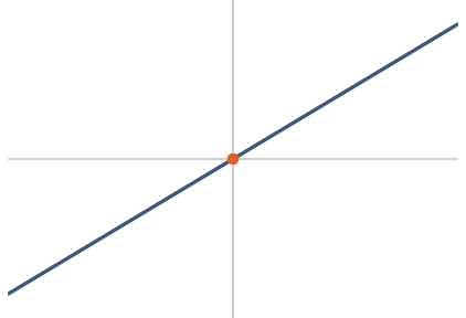
Figure 1
Somme et multiples restent sur la droite.
Une droite qui évite l’origine
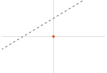
Figure 2
\(\mathbf{0}\) absent. Pas un sous-espace.
Le test le plus rapide
Réflexe \(\mathbf{0} \notin F\) suffit à conclure : \(F\) n’est pas un sous-espace.
Aucune autre vérification nécessaire.
Contre-exemples
Le premier quadrant \(\{x_1 \geqslant 0, \ x_2 \geqslant 0\}\).
\[\mathbf{u} = (1,1) \in F, \qquad (-1)\,\mathbf{u} = (-1,-1) \notin F\]
Le cercle unité, la réunion de deux droites distinctes.
Retour au point de départ
Premier résultat L’ensemble des solutions de \(A\mathbf{x} = \mathbf{0}\) est un sous-espace vectoriel de \(\mathbb{R}^n\).
Son nom : le noyau de \(A\).
Et pour \(A\mathbf{x} = \mathbf{b}\) ?
\(\mathbf{b} \neq \mathbf{0}\) : \(\mathbf{0}\) n’est pas solution.
Jamais un sous-espace.
Une droite ou un plan translaté — la description paramétrique du cours 2.
Espace engendré
Définition
Toutes les combinaisons linéaires de \(\mathbf{v}_1, \dots, \mathbf{v}_p\).
\[\operatorname{Vect}(\mathbf{v}_1, \dots, \mathbf{v}_p) = \bigl\{\, \alpha_1\mathbf{v}_1 + \dots + \alpha_p\mathbf{v}_p \;\bigm|\; \alpha_i \in \mathbb{R} \,\bigr\}\]
Notation également rencontrée : \(\langle \mathbf{v}_1, \dots, \mathbf{v}_p \rangle\).
Toujours un sous-espace
Somme de deux combinaisons : une combinaison.
Multiple d’une combinaison : une combinaison.
Propriété \(\operatorname{Vect}(\mathbf{v}_1, \dots, \mathbf{v}_p)\) est le plus petit sous-espace contenant \(\mathbf{v}_1, \dots, \mathbf{v}_p\).
Un seul vecteur
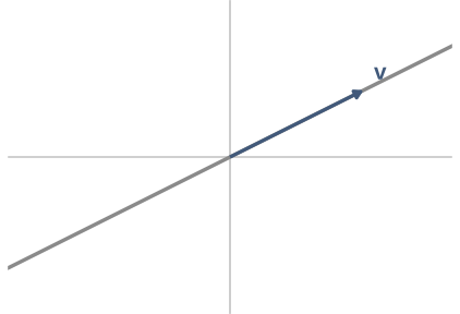
Figure 3
\(\operatorname{Vect}(\mathbf{v})\) : la droite portée par \(\mathbf{v}\), si \(\mathbf{v} \neq \mathbf{0}\).
Deux vecteurs du plan
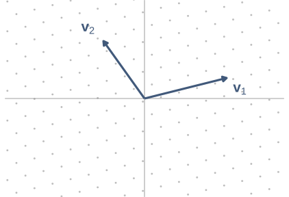
Figure 4
Non colinéaires : \(\operatorname{Vect}(\mathbf{v}_1, \mathbf{v}_2) = \mathbb{R}^2\).
Deux vecteurs colinéaires
\(\mathbf{v}_2 = 3\mathbf{v}_1\) :
\[\operatorname{Vect}(\mathbf{v}_1, \mathbf{v}_2) = \operatorname{Vect}(\mathbf{v}_1)\]
Une droite, pas un plan. Le second vecteur n’apporte rien.
Les colonnes d’une matrice
\(\operatorname{Vect}\) des colonnes de \(A\) : l’image de \(A\).
\[\operatorname{Im}(A) = \operatorname{Vect}(\mathbf{a}_1, \dots, \mathbf{a}_n) = \{\, A\mathbf{x} \mid \mathbf{x} \in \mathbb{R}^n \,\}\]
Reformulation du cours 3 \(A\mathbf{x} = \mathbf{b}\) compatible \(\iff \mathbf{b} \in \operatorname{Im}(A)\).
Deux sous-espaces pour une matrice
| Vit dans | Décrit | |
|---|---|---|
| Noyau \(\operatorname{Ker}(A)\) | \(\mathbb{R}^n\) | les solutions de \(A\mathbf{x}=\mathbf{0}\) |
| Image \(\operatorname{Im}(A)\) | \(\mathbb{R}^m\) | les \(\mathbf{b}\) atteignables |
Unicité d’un côté, existence de l’autre.
Familles génératrices
Définition
\((\mathbf{v}_1, \dots, \mathbf{v}_p)\) engendre \(F\) si tout vecteur de \(F\) est une combinaison linéaire des \(\mathbf{v}_i\).
\[F = \operatorname{Vect}(\mathbf{v}_1, \dots, \mathbf{v}_p)\]
Exemple canonique
\[ \mathbf{e}_1 = \begin{pmatrix} 1 \\ 0 \\ 0 \end{pmatrix}, \quad \mathbf{e}_2 = \begin{pmatrix} 0 \\ 1 \\ 0 \end{pmatrix}, \quad \mathbf{e}_3 = \begin{pmatrix} 0 \\ 0 \\ 1 \end{pmatrix} \]
Famille génératrice de \(\mathbb{R}^3\) : tout \(\mathbf{x}\) vaut \(x_1\mathbf{e}_1 + x_2\mathbf{e}_2 + x_3\mathbf{e}_3\).
Une question pratique
\(\mathbf{b} \in \operatorname{Vect}(\mathbf{v}_1, \dots, \mathbf{v}_p)\) ?
Traduction Une question d’appartenance devient un système linéaire. Le pivot de Gauss répond.
Ajouter sans rien gagner
Une famille génératrice reste génératrice après ajout d’un vecteur.
\[\operatorname{Vect}(\mathbf{v}_1, \dots, \mathbf{v}_p) = \operatorname{Vect}(\mathbf{v}_1, \dots, \mathbf{v}_p, \mathbf{w}) \iff \mathbf{w} \in \operatorname{Vect}(\mathbf{v}_1, \dots, \mathbf{v}_p)\]
D’où la question inverse : quels vecteurs sont superflus ?
Indépendance linéaire
Définition
\((\mathbf{v}_1, \dots, \mathbf{v}_p)\) est libre si la seule combinaison linéaire nulle est la combinaison triviale.
\[\alpha_1\mathbf{v}_1 + \dots + \alpha_p\mathbf{v}_p = \mathbf{0} \ \Longrightarrow \ \alpha_1 = \dots = \alpha_p = 0\]
Sinon : famille liée.
Deux emplois du mot « libre »
Variable libre — cours 2. Une inconnue dont la colonne ne porte pas de pivot.
Famille libre — ici. Des vecteurs dont aucun n’est superflu.
Homonymie assumée Deux notions sans rapport, un même adjectif. L’usage est établi ; la vigilance s’impose.
Le lien, malgré tout
Colonnes de \(A\) liées \(\iff\) \(A\mathbf{x} = \mathbf{0}\) a une solution non triviale.
\(\iff\) le système possède au moins une variable libre.
\[(\mathbf{a}_1, \dots, \mathbf{a}_n) \ \text{liée} \iff \operatorname{Ker}(A) \neq \{\mathbf{0}\}\]
Les deux mots se rencontrent dans la même phrase, sans se confondre.
Méthode
Liberté d’une famille : un système homogène à résoudre.
Critère par le pivot Famille libre \(\iff\) autant de pivots que de vecteurs.
\[(\mathbf{v}_1, \dots, \mathbf{v}_p) \ \text{libre} \iff r = p\]
Un vecteur
\((\mathbf{v})\) libre \(\iff \mathbf{v} \neq \mathbf{0}\).
\[\alpha \mathbf{v} = \mathbf{0} \ \text{ et } \ \mathbf{v} \neq \mathbf{0} \ \Longrightarrow \ \alpha = 0\]
Deux vecteurs
\((\mathbf{v}_1, \mathbf{v}_2)\) liée \(\iff\) colinéaires.
Attention Au-delà de deux vecteurs, la colinéarité deux à deux ne suffit plus. Trois vecteurs peuvent être liés sans qu’aucune paire ne le soit.
Familles nécessairement liées
Une famille contenant \(\mathbf{0}\).
\[1 \cdot \mathbf{0} + 0 \cdot \mathbf{v}_2 + \dots + 0 \cdot \mathbf{v}_p = \mathbf{0}\]
Une famille de plus de \(n\) vecteurs dans \(\mathbb{R}^n\).
\[p > n \ \Longrightarrow \ (\mathbf{v}_1, \dots, \mathbf{v}_p) \ \text{liée}\]
Pourquoi
\(p\) vecteurs de \(\mathbb{R}^n\) : un système homogène à \(n\) équations et \(p\) inconnues.
\(p > n\) : au plus \(n\) pivots, donc au moins une variable libre.
Une solution non triviale existe.
Reformulation
Vecteur superflu Famille liée \(\iff\) au moins un vecteur est combinaison linéaire des autres.
Le retirer ne change pas l’espace engendré.
Deux exigences opposées
Trop peu, trop
Génératrice — assez de vecteurs pour atteindre tout \(F\).
Libre — pas de vecteur superflu.
\[\text{génératrice} : \ \operatorname{Vect}(\mathbf{v}_1,\dots,\mathbf{v}_p) = F \qquad \text{libre} : \ \text{aucun } \mathbf{v}_i \ \text{redondant}\]
Deux réglages
Ajouter un vecteur : aide à engendrer, menace la liberté.
Retirer un vecteur : préserve la liberté, menace la génération.
Le point d’équilibre Une famille à la fois libre et génératrice : ni trop, ni trop peu.
Trois vecteurs de \(\mathbb{R}^3\)
\[ \mathbf{v}_1 = \begin{pmatrix} 1 \\ 0 \\ 1 \end{pmatrix}, \qquad \mathbf{v}_2 = \begin{pmatrix} 0 \\ 1 \\ 1 \end{pmatrix}, \qquad \mathbf{v}_3 = \begin{pmatrix} 1 \\ 1 \\ 2 \end{pmatrix} \]
Libre ? \(\mathbf{v}_3 = \mathbf{v}_1 + \mathbf{v}_2\) : famille liée.
Génératrice de \(\mathbb{R}^3\) ? \(\operatorname{Vect}(\mathbf{v}_1,\mathbf{v}_2,\mathbf{v}_3) = \operatorname{Vect}(\mathbf{v}_1,\mathbf{v}_2)\) : un plan.
Deux pivots pour trois vecteurs, dans \(\mathbb{R}^3\) : ni libre, ni génératrice.
Le même exemple, deux appartenances
\[ \operatorname{Vect}(\mathbf{v}_1, \mathbf{v}_2) = \bigl\{\, (a,\ b,\ a+b) \;\bigm|\; a, b \in \mathbb{R} \,\bigr\} \]
\[\begin{pmatrix} 2 \\ 1 \\ 3 \end{pmatrix} = 2\mathbf{v}_1 + \mathbf{v}_2 \ \in \operatorname{Vect}\]
\[\begin{pmatrix} 1 \\ 1 \\ 1 \end{pmatrix} : \quad a = 1, \ b = 1 \ \Longrightarrow \ a + b = 2 \neq 1 \quad \Longrightarrow \ \notin \operatorname{Vect}\]
Une troisième coordonnée imposée par les deux premières : l’équation du plan.
Récapitulatif
| Notion | Définition | Système | Verdict par le pivot |
|---|---|---|---|
| Sous-espace \(F\) | stable par combinaison | — | \(\mathbf{0} \notin F\) : non |
| \(\operatorname{Vect}(\mathbf{v}_1,\dots,\mathbf{v}_p)\) | toutes les combinaisons | — | toujours un sous-espace |
| \(\mathbf{b}\) atteignable ? | \(\mathbf{b} \in \operatorname{Vect}\) | \(A\mathbf{x} = \mathbf{b}\) | système compatible |
| Génératrice de \(\mathbb{R}^m\) | \(\operatorname{Vect} = \mathbb{R}^m\) | \(A\mathbf{x} = \mathbf{b}\), tout \(\mathbf{b}\) | un pivot par ligne : \(r = m\) |
| Libre | seule combinaison nulle triviale | \(A\mathbf{x} = \mathbf{0}\) | un pivot par colonne : \(r = p\) |
Une symétrie Engendrer se lit sur les lignes, être libre sur les colonnes. Le même calcul répond aux deux.